Multiple and logistic regression

class: center, middle, inverse, title-slide

# Multiple and logistic regression
### 2021/04/13

---

class: inverse, middle, center
# Linear regression - a (brief) recap

---
# Linear regression

.pull-left[

```
## `geom_smooth()` using formula 'y ~ x'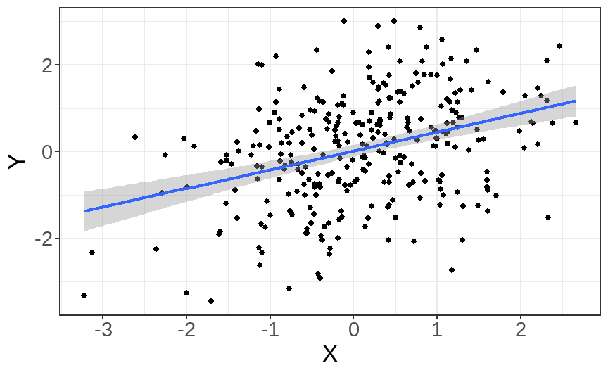
```
![](3-generalized-linear-models_files/figure-html/examp-lm-1.png)
]
.pull-right[
Our job is to figure out the mathematical relationship between our *predictor(s)* and our *outcome*.

$$ Y = b_0 + b_1X_i + \varepsilon_i $$
]

---
# Linear regression

$$ Y = b_0 + b_1X_i + \varepsilon_i $$

---
# Linear regression

$$ \color{red}Y = \color{#F6893D}{b_0} + \color{#FEBC38}{b_1}\color{blue}{X_i} + \color{green}{\varepsilon_i} $$

.red[
Y - The outcome - the dependent variable.
]

.brown[
`$b_0$` - The *intercept*. This is the value of `$Y$` when `$X$` = 0.
]

.orange[
`$b_1$` - The regression coefficients. This describes the steepness of the relationship between the outcome and *slope(s)*.
]

.blue[
`$X_i$` - The predictors - our independent variables.
]

.green[
`$\varepsilon_i$` - The *random error* - variability in our dependent variable that is not explained by our predictors. 
]

---
class: inverse, middle, center
# Regression assumptions

---
# Regression assumptions

Linear regression has a number of assumptions:

- Normally distributed errors

- Homoscedasticity (of errors)

- Independence of errors

- Linearity

- No perfect multicollinearity

---
# Normally distributed errors

.pull-left[
<img src="3-generalized-linear-models_files/figure-html/unnamed-chunk-1-1.png" width="432" />
]

.pull-right[
The *errors*, `$\varepsilon_i$`, are the variance left over after your model is fit.

An example like that on the left is what you want to see!

There is no clear pattern; the dots are evenly distributed around zero.
]

---
# Skewed errors

.pull-left[
<img src="3-generalized-linear-models_files/figure-html/unnamed-chunk-2-1.png" width="432" />
]
.pull-right[
In contrast, the residuals on the left are skewed.

This most often happens with data that are *bounded*. For example, *reaction times* cannot be below zero; negative values are impossible.
]

---
# Checking assumptions

.pull-left[
The `performance` package has a very handy function called `check_model()`, which shows a variety of ways of checking the assumptions all at once.

```r
library(performance)
check_model(test_skew)
```
]
.pull-right[
![](3-generalized-linear-models_files/figure-html/chck-mod-1.png)
]

---
# Checking assumptions

.pull-left[

You can follow up suspicious looking plots with individual functions like `check_normality()`, which uses `shapiro.test()` to check the residuals and also provides nice plots.

Rely on the plots more than significance tests...

```r
plot(check_normality(test_skew),
     type = "qq")
```

```
## Warning: Non-normality of residuals detected (p < .001).
```
]

.pull-right[
![](3-generalized-linear-models_files/figure-html/chck-norm-1.png)
]

---
# So, about violated assumptions? 😱

1) We can think about [transformations](https://craddm.github.io/resmethods/slides/Week-23-messy-data.html?panelset3=the-data2&panelset4=with-outliers2&panelset5=right-tailed2#30) 😱

2) We could consider *non-parametric stats* - things like `wilcox.test()`, `friedman.test()`, `kruskal.test()`, all of which are based on rank transformations and thus are really more like point 1 😱

3) We should think about **why** the assumptions might be violated. Is this just part of how the data is *generated*? 🤔

---
class: center, middle, inverse
# Generalized Linear Models

---
# Distributional families

.pull-left[
<img src="3-generalized-linear-models_files/figure-html/hypothetical-norm-1.png" width="432" />
]
.pull-right[
The *normal* distribution can also be called the *Gaussian* distribution.

The linear regression models we've used so far assume a *Gaussian* distribution of errors.
]

---
# Generalized linear models

A *Generalized Linear Model* - fit with `glm()` - allows you to specify what type of family of probability distributions the data are drawn from. 
.panelset[
.panel[.panel-name[The data]

```r
skewed_var <- rgamma(300, 1)
hist(skewed_var)
```

<img src="3-generalized-linear-models_files/figure-html/unnamed-chunk-3-1.png" width="432" />
]
.panel[.panel-name[With lm]

```r
lm(skewed_var ~ X1 + X2)
```

```
## 
## Call:
## lm(formula = skewed_var ~ X1 + X2)
## 
## Coefficients:
## (Intercept)           X1           X2  
##     0.99775     -0.04337      0.04234
```
]
.panel[.panel-name[With glm]

```r
glm(skewed_var ~ X1 + X2, family = "gaussian")
```

```
## 
## Call:  glm(formula = skewed_var ~ X1 + X2, family = "gaussian")
## 
## Coefficients:
## (Intercept)           X1           X2  
##     0.99775     -0.04337      0.04234  
## 
## Degrees of Freedom: 299 Total (i.e. Null);  297 Residual
## Null Deviance:	    268.9 
## Residual Deviance: 267.8 	AIC: 825.3
```
]
]

---
# Categorical outcome variables

Suppose you have a *discrete*, *categorical* outcome.

Examples of categorical outcomes:
- correct or incorrect answer
- person commits an offence or does not

Examples of counts:
- Number of items successfully recalled
- Number of offences committed

---
# The binomial distribution

A coin only has two sides: heads or tails.

Assuming the coin is fair, the probability - `$P$` - that it lands on *heads* is *.5*. So the probability it lands on *tails* - `$1 - P$` is also *.5*.

This type of variable is called a **Bernoulli random variable**.

If you toss the coin many times, the count of how many heads and how many tails occur is called a **binomial distribution**.

---
# Binomial distribution

If we throw the coin 100 times, how many times do we get tails?

```r
coin_flips <- rbinom(n = 100, size = 1, prob = 0.5)
qplot(coin_flips)
```

---
# Binomial distribution

What happens if we try to model individual coin flips with `lm()`?

```r
coin_flips <- rbinom(n = 100, size = 1, prob = 0.5)
x3 <- rnorm(100) # this is just a random variable for the purposes of demonstration!
check_model(lm(coin_flips ~ x3))
```

---
# Logistic regression

We get `glm()` to model a `binomial` distribution by specifying the *binomial* family.

```r
coin_flips <- rbinom(n = 100, size = 1, prob = 0.5)
glm(coin_flips ~ 1,
    family = binomial(link = "logit"))
```

```
## 
## Call:  glm(formula = coin_flips ~ 1, family = binomial(link = "logit"))
## 
## Coefficients:
## (Intercept)  
##    -0.04001  
## 
## Degrees of Freedom: 99 Total (i.e. Null);  99 Residual
## Null Deviance:	    138.6 
## Residual Deviance: 138.6 	AIC: 140.6
```

---
# Logistic regression

.pull-left[
The *logit* transformation is used to *link* our predictors to our discrete outcome variable.

It helps us constrain the influence of our predictors to the range 0-1, and account for the change in *variance* with probability.
]

.pull-right[
<img src="3-generalized-linear-models_files/figure-html/logit-curve-1.png" width="432" />
]

---
# Logistic regression

.pull-left[
As probabilities approach zero or one, the range of possible values *decreases*.

Thus, the influence of predictors on the *response scale* must also decrease as we reach one or zero.
]
.pull-right[
![](3-generalized-linear-models_files/figure-html/logit-curve-1.png)
]

---
# Logistic regression

$$ \color{red}{P(Y)} = \frac{1}{1 + e^-(b_0 + b_1X_1 + \varepsilon_i)} $$

.red[
`$P(Y)$` - The *probability* of the outcome happening.
]

---
# Logistic regression

$$ \color{red}{P(Y)} = \frac{\color{green}{1}}{\color{green}{1 + e^-(b_0 + b_1X_1 + \varepsilon_i)}} $$

.red[
`$P(Y)$` - The *probability* of the outcome happening.
]
.green[
`$\frac{1}{1 + e^-(...)}$` - The *log-odds* (logits) of the predictors.
]

---
# Odds ratios and log odds

**Odds** are the ratio of one outcome versus the others. e.g. The odds of a randomly chosen day being a Friday are 1 to 6 (or 1/6 = .17)

**Log odds** are the *natural log* of the odds:

`$$log(\frac{p}{1-p})$$`

The coefficients we get out are *log-odds* - they can be hard to interpret on their own.

```r
coef(glm(coin_flips ~ 1, family = binomial(link = "logit")))
```

```
## (Intercept) 
## -0.04000533
```

---
# Odds ratios and log odds

If we exponeniate them, we get the *odds ratios* back.

```r
exp(coef(glm(coin_flips ~ 1, family = binomial(link = "logit"))))
```

```
## (Intercept) 
##   0.9607843
```

So this one is roughly 1:1 heads and tails! But there's a nicer way to figure it out...

---
class: inverse, middle, center
# Taking penalties

![](images/terry-penalty.gif)

---
# Taking penalties

What's the probability that a particular penalty will be scored?

```
##   PSWQ Anxious Previous         Scored
## 1   18      21       56 Scored Penalty
## 2   17      32       35 Scored Penalty
## 3   16      34       35 Scored Penalty
## 4   14      40       15 Scored Penalty
## 5    5      24       47 Scored Penalty
## 6    1      15       67 Scored Penalty
```

- **PSWQ** = Penn State Worry Questionnaire
- **Anxiety** = State Anxiety
- **Previous** = Number of penalties scored previously

---
# Taking penalties

```r
pens <- glm(Scored ~ PSWQ + Anxious + Previous,
            family = binomial(link = "logit"),
            data = penalties)
pens
```

```
## 
## Call:  glm(formula = Scored ~ PSWQ + Anxious + Previous, family = binomial(link = "logit"), 
##     data = penalties)
## 
## Coefficients:
## (Intercept)         PSWQ      Anxious     Previous  
##    -11.4926      -0.2514       0.2758       0.2026  
## 
## Degrees of Freedom: 74 Total (i.e. Null);  71 Residual
## Null Deviance:	    103.6 
## Residual Deviance: 47.42 	AIC: 55.42
```

---

```
## 
## Call:
## glm(formula = Scored ~ PSWQ + Anxious + Previous, family = binomial(link = "logit"), 
##     data = penalties)
## 
## Deviance Residuals: 
##      Min        1Q    Median        3Q       Max  
## -2.31374  -0.35996   0.08334   0.53860   1.61380  
## 
## Coefficients:
##              Estimate Std. Error z value Pr(>|z|)   
## (Intercept) -11.49256   11.80175  -0.974  0.33016   
*## PSWQ         -0.25137    0.08401  -2.992  0.00277 **
## Anxious       0.27585    0.25259   1.092  0.27480   
## Previous      0.20261    0.12932   1.567  0.11719   
## ---
## Signif. codes:  0 '***' 0.001 '**' 0.01 '*' 0.05 '.' 0.1 ' ' 1
## 
## (Dispersion parameter for binomial family taken to be 1)
## 
##     Null deviance: 103.638  on 74  degrees of freedom
## Residual deviance:  47.416  on 71  degrees of freedom
## AIC: 55.416
## 
## Number of Fisher Scoring iterations: 6
```

---
# The response scale and the link scale

The model is fit on the *link* scale.

The coefficients returned by the GLM are in *logits*, or *log-odds*.

```r
coef(pens)
```

```
## (Intercept)        PSWQ     Anxious    Previous 
## -11.4925608  -0.2513693   0.2758489   0.2026082
```

How do we interpret them?

---
# Converting logits to odds ratios

```r
coef(pens)[2:4]
```

```
##       PSWQ    Anxious   Previous 
## -0.2513693  0.2758489  0.2026082
```

We can *exponentiate* the log-odds using the **exp()** function.

```r
exp(coef(pens)[2:4])
```

```
##      PSWQ   Anxious  Previous 
## 0.7777351 1.3176488 1.2245925
```

---
# Odds ratios

An odds ratio greater than 1 means that the odds of an outcome increase.

An odds ratio less than 1 means that the odds of an outcome decrease.

```r
exp(coef(pens)[2:4])
```

```
##      PSWQ   Anxious  Previous 
## 0.7777351 1.3176488 1.2245925
```

From this table, it looks like the odds of scoring a penalty decrease with increases in PSWQ but increase with increases in State Anxiety or Previous scoring rates.

---
# The response scale

The *response* scale is even *more* intuitive. It makes predictions using the *original* units. For a binomial distribution, that's *probabilities*. We can generate probabilities using the **predict()** function.

```r
penalties$prob <- predict(pens, type = "response")
head(penalties)
```

```
##   PSWQ Anxious Previous         Scored      prob
## 1   18      21       56 Scored Penalty 0.7542999
## 2   17      32       35 Scored Penalty 0.5380797
## 3   16      34       35 Scored Penalty 0.7222563
## 4   14      40       15 Scored Penalty 0.2811731
## 5    5      24       47 Scored Penalty 0.9675024
## 6    1      15       67 Scored Penalty 0.9974486
```

---
# Model predictions

Note that these model predictions *don't need to use the original data*. Let's see how the probability of scoring changes as `PSWQ` increases.

.panelset[
.panel[.panel-name[Create new data]

```r
new_dat <- 
  tibble::tibble(PSWQ = seq(0, 30, by = 2),
                 Anxious = mean(penalties$Anxious),
                 Previous = mean(penalties$Previous))
```
]
.panel[.panel-name[Make predictions]

```r
new_dat$probs <-
  predict(pens,
          newdata = new_dat,
          type = "response")
```
]
.panel[.panel-name[Plot predictions]
.pull-left[

```r
ggplot(new_dat, aes(x = PSWQ, y = probs)) +
  geom_point() +
  geom_line()
```
]
.pull-right[
![](3-generalized-linear-models_files/figure-html/prob-fig-1.png)
]
]
]

---
# Model predictions

Imagine you wanted to the probability of scoring for somebody with a PSWQ score of 7, an Anxious rating of 12, and a Previous scoring record of 34.

.panelset[
.panel[.panel-name[Make the data]

```r
new_dat <- tibble::tibble(PSWQ = 7,
                          Anxious = 22,
                          Previous = 34)
```
]
.panel[.panel-name[Predict log-odds]

```r
predict(pens, new_dat)
```

```
##          1 
## -0.2947909
```
]
.panel[.panel-name[Predict odds]

```r
exp(predict(pens, new_dat))
```

```
##         1 
## 0.7446873
```
]
.panel[.panel-name[Predict probabilities]

```r
predict(pens, new_dat, type = "response")
```

```
##         1 
## 0.4268314
```
]
]

---
# Plotting

.pull-left[

The **sjPlot** package has some excellent built in plotting tools - try the **plot_model()** function.

```r
library(sjPlot)
plot_model(pens,
           type = "pred",
           terms = "PSWQ")
```

```
## Data were 'prettified'. Consider using `terms="PSWQ [all]"` to get smooth plots.
```
]
.pull-right[
![](3-generalized-linear-models_files/figure-html/sj-plot-1.png)
]

---
# Results tables

```r
sjPlot::tab_model(pens)
```

<table style="border-collapse:collapse; border:none;">
<tr>
<th style="border-top: double; text-align:center; font-style:normal; font-weight:bold; padding:0.2cm;  text-align:left; ">&nbsp;</th>
<th colspan="3" style="border-top: double; text-align:center; font-style:normal; font-weight:bold; padding:0.2cm; ">Scored</th>
</tr>
<tr>
<td style=" text-align:center; border-bottom:1px solid; font-style:italic; font-weight:normal;  text-align:left; ">Predictors</td>
<td style=" text-align:center; border-bottom:1px solid; font-style:italic; font-weight:normal;  ">Odds Ratios</td>
<td style=" text-align:center; border-bottom:1px solid; font-style:italic; font-weight:normal;  ">CI</td>
<td style=" text-align:center; border-bottom:1px solid; font-style:italic; font-weight:normal;  ">p</td>
</tr>
<tr>
<td style=" padding:0.2cm; text-align:left; vertical-align:top; text-align:left; ">(Intercept)</td>
<td style=" padding:0.2cm; text-align:left; vertical-align:top; text-align:center;  ">0.00</td>
<td style=" padding:0.2cm; text-align:left; vertical-align:top; text-align:center;  ">0.00&nbsp;&ndash;&nbsp;64258.63</td>
<td style=" padding:0.2cm; text-align:left; vertical-align:top; text-align:center;  ">0.330</td>
</tr>
<tr>
<td style=" padding:0.2cm; text-align:left; vertical-align:top; text-align:left; ">PSWQ</td>
<td style=" padding:0.2cm; text-align:left; vertical-align:top; text-align:center;  ">0.78</td>
<td style=" padding:0.2cm; text-align:left; vertical-align:top; text-align:center;  ">0.64&nbsp;&ndash;&nbsp;0.90</td>
<td style=" padding:0.2cm; text-align:left; vertical-align:top; text-align:center;  "><strong>0.003</strong></td>
</tr>
<tr>
<td style=" padding:0.2cm; text-align:left; vertical-align:top; text-align:left; ">Anxious</td>
<td style=" padding:0.2cm; text-align:left; vertical-align:top; text-align:center;  ">1.32</td>
<td style=" padding:0.2cm; text-align:left; vertical-align:top; text-align:center;  ">0.81&nbsp;&ndash;&nbsp;2.24</td>
<td style=" padding:0.2cm; text-align:left; vertical-align:top; text-align:center;  ">0.275</td>
</tr>
<tr>
<td style=" padding:0.2cm; text-align:left; vertical-align:top; text-align:left; ">Previous</td>
<td style=" padding:0.2cm; text-align:left; vertical-align:top; text-align:center;  ">1.22</td>
<td style=" padding:0.2cm; text-align:left; vertical-align:top; text-align:center;  ">0.96&nbsp;&ndash;&nbsp;1.61</td>
<td style=" padding:0.2cm; text-align:left; vertical-align:top; text-align:center;  ">0.117</td>
</tr>
<tr>
<td style=" padding:0.2cm; text-align:left; vertical-align:top; text-align:left; padding-top:0.1cm; padding-bottom:0.1cm; border-top:1px solid;">Observations</td>
<td style=" padding:0.2cm; text-align:left; vertical-align:top; padding-top:0.1cm; padding-bottom:0.1cm; text-align:left; border-top:1px solid;" colspan="3">75</td>
</tr>
<tr>
<td style=" padding:0.2cm; text-align:left; vertical-align:top; text-align:left; padding-top:0.1cm; padding-bottom:0.1cm;">R<sup>2</sup> Tjur</td>
<td style=" padding:0.2cm; text-align:left; vertical-align:top; padding-top:0.1cm; padding-bottom:0.1cm; text-align:left;" colspan="3">0.594</td>
</tr>

</table>

---
class: inverse, middle, center
# The Titanic dataset

![](images/titanic.gif)

---
class: inverse, middle, center
# The Titanic dataset

![](images/rose84.gif)
---
# The Titanic dataset

```r
head(full_titanic)
```

```
## # A tibble: 6 x 12
##   PassengerId Survived Pclass Name    Sex     Age SibSp Parch Ticket  Fare Cabin
##         <dbl>    <dbl>  <dbl> <chr>   <chr> <dbl> <dbl> <dbl> <chr>  <dbl> <chr>
## 1           1        0      3 Braund~ male     22     1     0 A/5 2~  7.25 <NA> 
## 2           2        1      1 Cuming~ fema~    38     1     0 PC 17~ 71.3  C85  
## 3           3        1      3 Heikki~ fema~    26     0     0 STON/~  7.92 <NA> 
## 4           4        1      1 Futrel~ fema~    35     1     0 113803 53.1  C123 
## 5           5        0      3 Allen,~ male     35     0     0 373450  8.05 <NA> 
## 6           6        0      3 Moran,~ male     NA     0     0 330877  8.46 <NA> 
## # ... with 1 more variable: Embarked <chr>
```

Downloaded from [Kaggle](https://www.kaggle.com/c/titanic)

---
# The Titanic dataset

![](images/titanic.png)

---
# The Titanic dataset

.pull-left[

```r
full_titanic %>% 
  group_by(Survived,
           Sex) %>%
  count()
```

```
## # A tibble: 4 x 3
## # Groups:   Survived, Sex [4]
##   Survived Sex        n
##      <dbl> <chr>  <int>
## 1        0 female    81
## 2        0 male     468
## 3        1 female   233
## 4        1 male     109
```
]
.pull-right[

```r
full_titanic %>%
  group_by(Sex) %>%
  summarise(p = mean(Survived),
            Y = sum(Survived),
            N = n())
```

```
## # A tibble: 2 x 4
##   Sex        p     Y     N
##   <chr>  <dbl> <dbl> <int>
## 1 female 0.742   233   314
## 2 male   0.189   109   577
```
]

---
# The Titanic dataset

```
## 
## Call:
## glm(formula = Survived ~ Age + Pclass, family = binomial(), data = full_titanic)
## 
## Deviance Residuals: 
##     Min       1Q   Median       3Q      Max  
## -2.1524  -0.8466  -0.6083   1.0031   2.3929  
## 
## Coefficients:
##              Estimate Std. Error z value Pr(>|z|)    
## (Intercept)  2.296012   0.317629   7.229 4.88e-13 ***
## Age         -0.041755   0.006736  -6.198 5.70e-10 ***
## Pclass2     -1.137533   0.237578  -4.788 1.68e-06 ***
## Pclass3     -2.469561   0.240182 -10.282  < 2e-16 ***
## ---
## Signif. codes:  0 '***' 0.001 '**' 0.01 '*' 0.05 '.' 0.1 ' ' 1
## 
## (Dispersion parameter for binomial family taken to be 1)
## 
##     Null deviance: 964.52  on 713  degrees of freedom
## Residual deviance: 827.16  on 710  degrees of freedom
##   (177 observations deleted due to missingness)
## AIC: 835.16
## 
## Number of Fisher Scoring iterations: 4
```

---
# The Titanic dataset

```r
library(emmeans)
emmeans(age_class,
        ~Age|Pclass,
        type = "response")
```

```
## Pclass = 1:
##   Age  prob     SE  df asymp.LCL asymp.UCL
##  29.7 0.742 0.0339 Inf     0.670     0.803
## 
## Pclass = 2:
##   Age  prob     SE  df asymp.LCL asymp.UCL
##  29.7 0.480 0.0394 Inf     0.403     0.557
## 
## Pclass = 3:
##   Age  prob     SE  df asymp.LCL asymp.UCL
##  29.7 0.196 0.0216 Inf     0.157     0.241
## 
## Confidence level used: 0.95 
## Intervals are back-transformed from the logit scale
```

---
# Some final notes on Generalized Linear Models

Today has focussed on **logistic** regression with *binomial* distributions.

But Generalized Linear Models can be expanded to deal with many different types of outcome variable!

e.g. 
*Counts* follow a Poisson distribution - use `family = "poisson"`

Ordinal variables (e.g. Likert scale) can be modelled using *cumulative logit* models (using the **ordinal** or **brms** packages).

---
#Suggested reading for categorical ordinal regression

[Liddell & Kruschke (2018). Analyzing ordinal data with metric models: What could possibly go Wrong?](https://www.sciencedirect.com/science/article/pii/S0022103117307746)

[Buerkner & Vuorre (2018). Ordinal Regression Models in Psychology: A Tutorial](https://psyarxiv.com/x8swp/)