class: center, middle, inverse, title-slide # Moderation and Mediation ### 2021/04/27 --- # Mediation and moderation In linear regression, we're looking to understand the relationship between *predictors* and *outcomes*. .pull-left[ 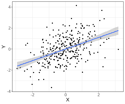 ] .pull-right[ 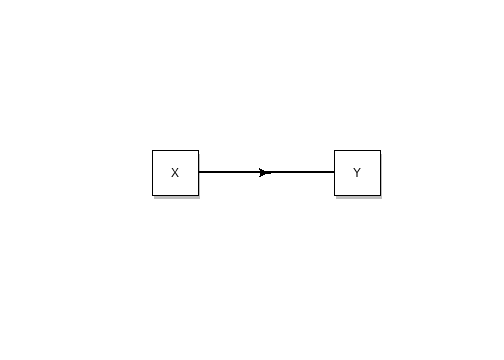<!-- --> ] --- class: inverse, center, middle # Moderation --- # Moderation Moderation is when the strength of the relationship between two variables depends on a third variable. .center[  ] --- # The *epi.bfi* dataset The `epi.bfi` dataset from the `psychTools` package ```r head(epi.bfi) ``` ``` ## epiE epiS epiImp epilie epiNeur bfagree bfcon bfext bfneur bfopen bdi ## 1 18 10 7 3 9 138 96 141 51 138 1 ## 2 16 8 5 1 12 101 99 107 116 132 7 ## 3 6 1 3 2 5 143 118 38 68 90 4 ## 4 12 6 4 3 15 104 106 64 114 101 8 ## 5 14 6 5 3 2 115 102 103 86 118 8 ## 6 6 4 2 5 15 110 113 61 54 149 5 ## traitanx stateanx ## 1 24 22 ## 2 41 40 ## 3 37 44 ## 4 54 40 ## 5 39 67 ## 6 51 38 ``` --- # Simple linear regression Let's model `bdi` (Beck Depression Inventory) as a function of `stateanx` (State Anxiety) ```r st_bdi <- lm(bdi ~ stateanx, data = epi.bfi) summary(st_bdi) ``` ``` ## ## Call: ## lm(formula = bdi ~ stateanx, data = epi.bfi) ## ## Residuals: ## Min 1Q Median 3Q Max ## -11.1115 -3.0603 -0.6826 2.2152 15.1130 ## ## Coefficients: ## Estimate Std. Error t value Pr(>|t|) ## (Intercept) -5.41988 1.09322 -4.958 1.39e-06 *** ## stateanx 0.30614 0.02637 11.611 < 2e-16 *** ## --- ## Signif. codes: 0 '***' 0.001 '**' 0.01 '*' 0.05 '.' 0.1 ' ' 1 ## ## Residual standard error: 4.592 on 229 degrees of freedom ## Multiple R-squared: 0.3706, Adjusted R-squared: 0.3678 ## F-statistic: 134.8 on 1 and 229 DF, p-value: < 2.2e-16 ``` --- # Multiple linear regression An additional predictor that we may find interesting is `epiNeur` - a measure of *neuroticism* from the *Eysenck Personality Inventory*. ```r st_neu <- lm(bdi ~ stateanx + epiNeur, data = epi.bfi) summary(st_neu) ``` ``` ## ## Call: ## lm(formula = bdi ~ stateanx + epiNeur, data = epi.bfi) ## ## Residuals: ## Min 1Q Median 3Q Max ## -9.7405 -2.5748 -0.5299 2.2841 11.7303 ## ## Coefficients: ## Estimate Std. Error t value Pr(>|t|) ## (Intercept) -6.32655 1.01061 -6.260 1.89e-09 *** ## stateanx 0.21526 0.02770 7.770 2.66e-13 *** ## epiNeur 0.43492 0.06493 6.698 1.63e-10 *** ## --- ## Signif. codes: 0 '***' 0.001 '**' 0.01 '*' 0.05 '.' 0.1 ' ' 1 ## ## Residual standard error: 4.207 on 228 degrees of freedom ## Multiple R-squared: 0.4741, Adjusted R-squared: 0.4694 ## F-statistic: 102.8 on 2 and 228 DF, p-value: < 2.2e-16 ``` --- # Adding interaction terms What if the effect of `stateanx` depends on the level of `epiNeur`? For example, people who score high on *neuroticism* might be more affected by *state anxiety* than people who are low on *neuroticism*. We add an interaction to our model using `:` between the two variables: ```r int_model <- lm(bdi ~ stateanx + epiNeur + stateanx:epiNeur, data = epi.bfi) ``` We can also use `*` instead of `+`. Thus, `stateanx * epiNeur` will give us the main effect of `stateanx`, the main effect of `epiNeur`, and the interaction between the two. --- # Moderation .pull-left[ <!-- --> ] .pull-right[ An interaction like this has *three* terms. There is a term for each of the main effects. There is also a term for the interaction, which is the *product* of the two main effects. ] --- ```r summary(int_model) ``` ``` ## ## Call: ## lm(formula = bdi ~ stateanx + epiNeur + stateanx:epiNeur, data = epi.bfi) ## ## Residuals: ## Min 1Q Median 3Q Max ## -12.0493 -2.2513 -0.4707 2.1135 11.9949 ## ## Coefficients: ## Estimate Std. Error t value Pr(>|t|) ## (Intercept) 0.06367 2.18559 0.029 0.9768 ## stateanx 0.03750 0.06062 0.619 0.5368 ## epiNeur -0.14765 0.18869 -0.782 0.4347 *## stateanx:epiNeur 0.01528 0.00466 3.279 0.0012 ** ## --- ## Signif. codes: 0 '***' 0.001 '**' 0.01 '*' 0.05 '.' 0.1 ' ' 1 ## ## Residual standard error: 4.12 on 227 degrees of freedom ## Multiple R-squared: 0.4978, Adjusted R-squared: 0.4912 ## F-statistic: 75.02 on 3 and 227 DF, p-value: < 2.2e-16 ``` --- # Interpreting the coefficients ```r coef(int_model) ``` ``` ## (Intercept) stateanx epiNeur stateanx:epiNeur ## 0.06367327 0.03750035 -0.14764857 0.01527977 ``` The coefficients tell you what the effect of a 1 unit increase in the variable has on the dependent variable. But the coefficients of the main effects (`stateanx` and `epiNeur`) are hard to interpret *in the presence of an interaction* unless the variables have been **centred**. --- # Interpreting the coefficients ```r coef(int_model) ``` ``` ## (Intercept) stateanx epiNeur stateanx:epiNeur ## 0.06367327 0.03750035 -0.14764857 0.01527977 ``` When the predictors are uncentred, these coefficients tell us (*take a deep breath*) - the effect of a 1 unit increase in `stateanx` when `epiNeur` is 0 - the effect of a 1 unit increase in `epiNeur` when `stateanx` is 0 - the difference between the effect of a 1 unit increase in `stateanx` when `epiNeur` is 0 and the increase in `stateanx` when `epiNeur` is 1, and the difference between the effect of a 1 unit the increase in `epiNeur` when `stateanx` is 0 and the increase in `epiNeur` when `stateanx` is 1 (or something like that) --- # Mean-centring We can use the `scale()` function to perform mean-centring, standardization, or both. ```r cent_model <- lm(bdi ~ scale(stateanx, scale = FALSE) * scale(epiNeur, scale = FALSE), data = epi.bfi) coef(cent_model) ``` ``` ## (Intercept) ## 6.35996006 ## scale(stateanx, scale = FALSE) ## 0.19658197 ## scale(epiNeur, scale = FALSE) ## 0.46122726 ## scale(stateanx, scale = FALSE):scale(epiNeur, scale = FALSE) ## 0.01527977 ``` ```r coef(st_neu) ``` ``` ## (Intercept) stateanx epiNeur ## -6.3265496 0.2152590 0.4349163 ``` --- ```r tab_model(st_neu, int_model) ``` <table style="border-collapse:collapse; border:none;"> <tr> <th style="border-top: double; text-align:center; font-style:normal; font-weight:bold; padding:0.2cm; text-align:left; "> </th> <th colspan="3" style="border-top: double; text-align:center; font-style:normal; font-weight:bold; padding:0.2cm; ">bdi</th> <th colspan="3" style="border-top: double; text-align:center; font-style:normal; font-weight:bold; padding:0.2cm; ">bdi</th> </tr> <tr> <td style=" text-align:center; border-bottom:1px solid; font-style:italic; font-weight:normal; text-align:left; ">Predictors</td> <td style=" text-align:center; border-bottom:1px solid; font-style:italic; font-weight:normal; ">Estimates</td> <td style=" text-align:center; border-bottom:1px solid; font-style:italic; font-weight:normal; ">CI</td> <td style=" text-align:center; border-bottom:1px solid; font-style:italic; font-weight:normal; ">p</td> <td style=" text-align:center; border-bottom:1px solid; font-style:italic; font-weight:normal; ">Estimates</td> <td style=" text-align:center; border-bottom:1px solid; font-style:italic; font-weight:normal; ">CI</td> <td style=" text-align:center; border-bottom:1px solid; font-style:italic; font-weight:normal; col7">p</td> </tr> <tr> <td style=" padding:0.2cm; text-align:left; vertical-align:top; text-align:left; ">(Intercept)</td> <td style=" padding:0.2cm; text-align:left; vertical-align:top; text-align:center; ">-6.33</td> <td style=" padding:0.2cm; text-align:left; vertical-align:top; text-align:center; ">-8.32 – -4.34</td> <td style=" padding:0.2cm; text-align:left; vertical-align:top; text-align:center; "><strong><0.001</td> <td style=" padding:0.2cm; text-align:left; vertical-align:top; text-align:center; ">0.06</td> <td style=" padding:0.2cm; text-align:left; vertical-align:top; text-align:center; ">-4.24 – 4.37</td> <td style=" padding:0.2cm; text-align:left; vertical-align:top; text-align:center; col7">0.977</td> </tr> <tr> <td style=" padding:0.2cm; text-align:left; vertical-align:top; text-align:left; ">stateanx</td> <td style=" padding:0.2cm; text-align:left; vertical-align:top; text-align:center; ">0.22</td> <td style=" padding:0.2cm; text-align:left; vertical-align:top; text-align:center; ">0.16 – 0.27</td> <td style=" padding:0.2cm; text-align:left; vertical-align:top; text-align:center; "><strong><0.001</td> <td style=" padding:0.2cm; text-align:left; vertical-align:top; text-align:center; ">0.04</td> <td style=" padding:0.2cm; text-align:left; vertical-align:top; text-align:center; ">-0.08 – 0.16</td> <td style=" padding:0.2cm; text-align:left; vertical-align:top; text-align:center; col7">0.537</td> </tr> <tr> <td style=" padding:0.2cm; text-align:left; vertical-align:top; text-align:left; ">epiNeur</td> <td style=" padding:0.2cm; text-align:left; vertical-align:top; text-align:center; ">0.43</td> <td style=" padding:0.2cm; text-align:left; vertical-align:top; text-align:center; ">0.31 – 0.56</td> <td style=" padding:0.2cm; text-align:left; vertical-align:top; text-align:center; "><strong><0.001</td> <td style=" padding:0.2cm; text-align:left; vertical-align:top; text-align:center; ">-0.15</td> <td style=" padding:0.2cm; text-align:left; vertical-align:top; text-align:center; ">-0.52 – 0.22</td> <td style=" padding:0.2cm; text-align:left; vertical-align:top; text-align:center; col7">0.435</td> </tr> <tr> <td style=" padding:0.2cm; text-align:left; vertical-align:top; text-align:left; ">stateanx * epiNeur</td> <td style=" padding:0.2cm; text-align:left; vertical-align:top; text-align:center; "></td> <td style=" padding:0.2cm; text-align:left; vertical-align:top; text-align:center; "></td> <td style=" padding:0.2cm; text-align:left; vertical-align:top; text-align:center; "></td> <td style=" padding:0.2cm; text-align:left; vertical-align:top; text-align:center; ">0.02</td> <td style=" padding:0.2cm; text-align:left; vertical-align:top; text-align:center; ">0.01 – 0.02</td> <td style=" padding:0.2cm; text-align:left; vertical-align:top; text-align:center; col7"><strong>0.001</strong></td> </tr> <tr> <td style=" padding:0.2cm; text-align:left; vertical-align:top; text-align:left; padding-top:0.1cm; padding-bottom:0.1cm; border-top:1px solid;">Observations</td> <td style=" padding:0.2cm; text-align:left; vertical-align:top; padding-top:0.1cm; padding-bottom:0.1cm; text-align:left; border-top:1px solid;" colspan="3">231</td> <td style=" padding:0.2cm; text-align:left; vertical-align:top; padding-top:0.1cm; padding-bottom:0.1cm; text-align:left; border-top:1px solid;" colspan="3">231</td> </tr> <tr> <td style=" padding:0.2cm; text-align:left; vertical-align:top; text-align:left; padding-top:0.1cm; padding-bottom:0.1cm;">R<sup>2</sup> / R<sup>2</sup> adjusted</td> <td style=" padding:0.2cm; text-align:left; vertical-align:top; padding-top:0.1cm; padding-bottom:0.1cm; text-align:left;" colspan="3">0.474 / 0.469</td> <td style=" padding:0.2cm; text-align:left; vertical-align:top; padding-top:0.1cm; padding-bottom:0.1cm; text-align:left;" colspan="3">0.498 / 0.491</td> </tr> </table> --- # Simple slopes .pull-left[ The `interact_plot()` function from the `interactions` package provides a nice way to visualize the interaction. We look at the steepness of the slope at different levels of one of the variables. ```r interact_plot(int_model, pred = stateanx, modx = epiNeur) ``` ] .pull-right[  ] --- # Simple slopes .pull-left[ We can also add individual data points using `plot.points = TRUE`. Confidence intervals can be added using `interval = TRUE`. ```r interact_plot(int_model, pred = stateanx, modx = epiNeur, plot.points = TRUE, interval = TRUE) ``` ] .pull-right[  ] --- # Simple slopes The interaction means that the *slope* of the effect of `stateanx` differs at different values of `epiNeur`. We can use the `sim_slopes()` function from `interactions` to statistically explore how `stateanx` varies as a function of `epiNeur`. ```r sim_slopes(int_model, pred = stateanx, modx = epiNeur, johnson_neyman = FALSE) ``` --- ``` ## SIMPLE SLOPES ANALYSIS ## ## Slope of stateanx when epiNeur = 5.51 (- 1 SD): ## ## Est. S.E. t val. p ## ------ ------ -------- ------ ## 0.12 0.04 3.09 0.00 ## ## Slope of stateanx when epiNeur = 10.41 (Mean): ## ## Est. S.E. t val. p ## ------ ------ -------- ------ ## 0.20 0.03 7.09 0.00 ## ## Slope of stateanx when epiNeur = 15.31 (+ 1 SD): ## ## Est. S.E. t val. p ## ------ ------ -------- ------ ## 0.27 0.03 8.46 0.00 ``` The slope of `stateanx` *increases* as `epiNeur` increases. --- # Johnson-Neyman plots ```r johnson_neyman(int_model, pred = stateanx, modx = epiNeur) ``` ``` ## JOHNSON-NEYMAN INTERVAL ## ## When epiNeur is OUTSIDE the interval [-24.37, 3.54], the slope of stateanx ## is p < .05. ## ## Note: The range of observed values of epiNeur is [0.00, 23.00] ```  --- class: inverse, center, middle # Mediation --- # Mediation Mediation refers to a situation in which the effect of a predictor is transmitted *through* another variable. .center[ 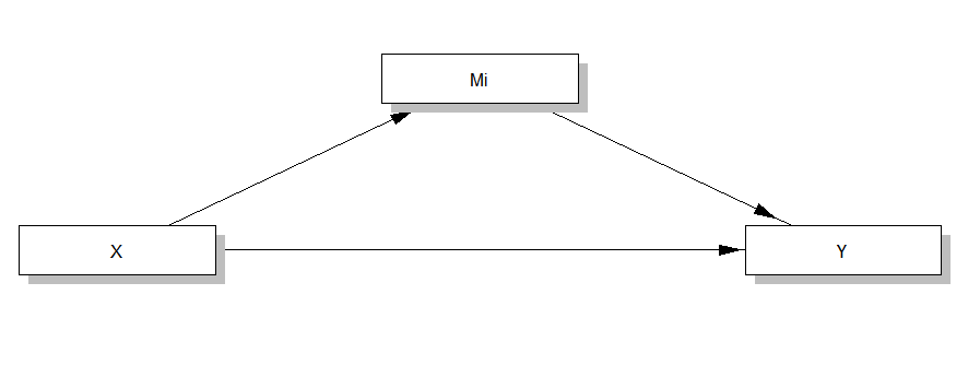 ] --- # Mediation In this example, *room temperature* predicts the *amount that people drink*; specifically, we'd expect that higher temperatures would increase drinking. .center[  ] --- # Mediation Nevertheless, it's possible that higher temperatures increase drinking *indirectly*: higher temperatures make people feel more *thirsty*, which in turn makes them *drink more*. .center[  ] --- # Mediation path diagram .pull-left[ <!-- --> ] .pull-right[ `\(a\)` - the effect of the IV on the mediator `\(b\)` - the effect of the mediator on the DV `\(c'\)` - the *direct* effect of the IV on the DV Missing here are path `\(c\)` - the *total* effect of the IV on the DV - and path `\(ab\)` - the *indirect* effect of the IV on the DV ] --- # Mediation as regression Baron & Kenny (1986) outline steps to estimate each *path* with regression. <!-- --> --- # The `estress` data ``` ## # A tibble: 5 x 7 ## tenure estress affect withdraw sex age ese ## <dbl> <dbl> <dbl> <dbl> <dbl> <dbl> <dbl> ## 1 1.67 6 2.6 3 1 51 5.33 ## 2 0.58 5 1 1 0 45 6.05 ## 3 0.58 5.5 2.4 3.66 1 42 5.26 ## 4 2 3 1.16 4.66 1 50 4.35 ## 5 5 4.5 1 4.33 1 48 4.86 ``` Pollack, J., VanEpps, E. M., & Hayes, A. F. (2012). The moderating role of social ties on entrepreneurs' depressed affect and withdrawal intentions in response to economic stress. Journal of Organizational Behavior, 33, 789-810. --- # Path *c* - the *total* effect This is the effect of the IV on the DV. ```r path_c <- lm(withdraw ~ estress, data = estress) summary(path_c) ``` ``` ## ## Call: ## lm(formula = withdraw ~ estress, data = estress) ## ## Residuals: ## Min 1Q Median 3Q Max ## -1.4547 -1.2302 -0.2022 0.7978 4.8820 ## ## Coefficients: ## Estimate Std. Error t value Pr(>|t|) ## (Intercept) 2.06187 0.26202 7.869 9.64e-14 *** *## estress 0.05612 0.05421 1.035 0.302 ## --- ## Signif. codes: 0 '***' 0.001 '**' 0.01 '*' 0.05 '.' 0.1 ' ' 1 ## ## Residual standard error: 1.247 on 260 degrees of freedom ## Multiple R-squared: 0.004105, Adjusted R-squared: 0.0002748 ## F-statistic: 1.072 on 1 and 260 DF, p-value: 0.3015 ``` --- # Path *a* This is the effect of the IV on the Mediator. ```r path_a <- lm(affect ~ estress, data = estress) summary(path_a) ``` ``` ## ## Call: ## lm(formula = affect ~ estress, data = estress) ## ## Residuals: ## Min 1Q Median 3Q Max ## -1.0095 -0.4195 -0.1609 0.2498 4.0278 ## ## Coefficients: ## Estimate Std. Error t value Pr(>|t|) ## (Intercept) 0.79936 0.14331 5.578 6.11e-08 *** *## estress 0.17288 0.02965 5.831 1.63e-08 *** ## --- ## Signif. codes: 0 '***' 0.001 '**' 0.01 '*' 0.05 '.' 0.1 ' ' 1 ## ## Residual standard error: 0.6819 on 260 degrees of freedom ## Multiple R-squared: 0.1156, Adjusted R-squared: 0.1122 ## F-statistic: 34 on 1 and 260 DF, p-value: 1.63e-08 ``` --- # Path *b* This is the effect of the mediator on the DV, controlling for the IV. ```r path_b <- lm(withdraw ~ affect, data = estress) summary(path_b) ``` ``` ## ## Call: ## lm(formula = withdraw ~ affect, data = estress) ## ## Residuals: ## Min 1Q Median 3Q Max ## -3.1028 -0.8919 -0.2092 0.8713 2.8713 ## ## Coefficients: ## Estimate Std. Error t value Pr(>|t|) ## (Intercept) 1.17416 0.17035 6.893 4.13e-11 *** *## affect 0.71772 0.09713 7.389 2.02e-12 *** ## --- ## Signif. codes: 0 '***' 0.001 '**' 0.01 '*' 0.05 '.' 0.1 ' ' 1 ## ## Residual standard error: 1.136 on 260 degrees of freedom ## Multiple R-squared: 0.1735, Adjusted R-squared: 0.1704 ## F-statistic: 54.6 on 1 and 260 DF, p-value: 2.02e-12 ``` --- # Path *c'* - the direct effect This checks whether the IV predicts the DV after controlling for the mediator. ```r path_c_dir <- lm(withdraw ~ affect + estress, data = estress) summary(path_c_dir) ``` ``` ## ## Call: ## lm(formula = withdraw ~ affect + estress, data = estress) ## ## Residuals: ## Min 1Q Median 3Q Max ## -3.1716 -0.9472 -0.2249 0.8490 2.9049 ## ## Coefficients: ## Estimate Std. Error t value Pr(>|t|) ## (Intercept) 1.44706 0.25201 5.742 2.61e-08 *** ## affect 0.76913 0.10306 7.463 1.29e-12 *** *## estress -0.07685 0.05239 -1.467 0.144 ## --- ## Signif. codes: 0 '***' 0.001 '**' 0.01 '*' 0.05 '.' 0.1 ' ' 1 ## ## Residual standard error: 1.133 on 259 degrees of freedom ## Multiple R-squared: 0.1804, Adjusted R-squared: 0.174 ## F-statistic: 28.49 on 2 and 259 DF, p-value: 6.528e-12 ``` --- # Is there mediation? Now that we've fit all these models, how do we work out if there is *mediation*? Does the effect of `estress` differ after controlling for `affect`? ```r tab_model(path_c, path_c_dir) ``` <table style="border-collapse:collapse; border:none;"> <tr> <th style="border-top: double; text-align:center; font-style:normal; font-weight:bold; padding:0.2cm; text-align:left; "> </th> <th colspan="3" style="border-top: double; text-align:center; font-style:normal; font-weight:bold; padding:0.2cm; ">withdraw</th> <th colspan="3" style="border-top: double; text-align:center; font-style:normal; font-weight:bold; padding:0.2cm; ">withdraw</th> </tr> <tr> <td style=" text-align:center; border-bottom:1px solid; font-style:italic; font-weight:normal; text-align:left; ">Predictors</td> <td style=" text-align:center; border-bottom:1px solid; font-style:italic; font-weight:normal; ">Estimates</td> <td style=" text-align:center; border-bottom:1px solid; font-style:italic; font-weight:normal; ">CI</td> <td style=" text-align:center; border-bottom:1px solid; font-style:italic; font-weight:normal; ">p</td> <td style=" text-align:center; border-bottom:1px solid; font-style:italic; font-weight:normal; ">Estimates</td> <td style=" text-align:center; border-bottom:1px solid; font-style:italic; font-weight:normal; ">CI</td> <td style=" text-align:center; border-bottom:1px solid; font-style:italic; font-weight:normal; col7">p</td> </tr> <tr> <td style=" padding:0.2cm; text-align:left; vertical-align:top; text-align:left; ">(Intercept)</td> <td style=" padding:0.2cm; text-align:left; vertical-align:top; text-align:center; ">2.06</td> <td style=" padding:0.2cm; text-align:left; vertical-align:top; text-align:center; ">1.55 – 2.58</td> <td style=" padding:0.2cm; text-align:left; vertical-align:top; text-align:center; "><strong><0.001</td> <td style=" padding:0.2cm; text-align:left; vertical-align:top; text-align:center; ">1.45</td> <td style=" padding:0.2cm; text-align:left; vertical-align:top; text-align:center; ">0.95 – 1.94</td> <td style=" padding:0.2cm; text-align:left; vertical-align:top; text-align:center; col7"><strong><0.001</td> </tr> <tr> <td style=" padding:0.2cm; text-align:left; vertical-align:top; text-align:left; ">estress</td> <td style=" padding:0.2cm; text-align:left; vertical-align:top; text-align:center; ">0.06</td> <td style=" padding:0.2cm; text-align:left; vertical-align:top; text-align:center; ">-0.05 – 0.16</td> <td style=" padding:0.2cm; text-align:left; vertical-align:top; text-align:center; ">0.302</td> <td style=" padding:0.2cm; text-align:left; vertical-align:top; text-align:center; ">-0.08</td> <td style=" padding:0.2cm; text-align:left; vertical-align:top; text-align:center; ">-0.18 – 0.03</td> <td style=" padding:0.2cm; text-align:left; vertical-align:top; text-align:center; col7">0.144</td> </tr> <tr> <td style=" padding:0.2cm; text-align:left; vertical-align:top; text-align:left; ">affect</td> <td style=" padding:0.2cm; text-align:left; vertical-align:top; text-align:center; "></td> <td style=" padding:0.2cm; text-align:left; vertical-align:top; text-align:center; "></td> <td style=" padding:0.2cm; text-align:left; vertical-align:top; text-align:center; "></td> <td style=" padding:0.2cm; text-align:left; vertical-align:top; text-align:center; ">0.77</td> <td style=" padding:0.2cm; text-align:left; vertical-align:top; text-align:center; ">0.57 – 0.97</td> <td style=" padding:0.2cm; text-align:left; vertical-align:top; text-align:center; col7"><strong><0.001</td> </tr> <tr> <td style=" padding:0.2cm; text-align:left; vertical-align:top; text-align:left; padding-top:0.1cm; padding-bottom:0.1cm; border-top:1px solid;">Observations</td> <td style=" padding:0.2cm; text-align:left; vertical-align:top; padding-top:0.1cm; padding-bottom:0.1cm; text-align:left; border-top:1px solid;" colspan="3">262</td> <td style=" padding:0.2cm; text-align:left; vertical-align:top; padding-top:0.1cm; padding-bottom:0.1cm; text-align:left; border-top:1px solid;" colspan="3">262</td> </tr> <tr> <td style=" padding:0.2cm; text-align:left; vertical-align:top; text-align:left; padding-top:0.1cm; padding-bottom:0.1cm;">R<sup>2</sup> / R<sup>2</sup> adjusted</td> <td style=" padding:0.2cm; text-align:left; vertical-align:top; padding-top:0.1cm; padding-bottom:0.1cm; text-align:left;" colspan="3">0.004 / 0.000</td> <td style=" padding:0.2cm; text-align:left; vertical-align:top; padding-top:0.1cm; padding-bottom:0.1cm; text-align:left;" colspan="3">0.180 / 0.174</td> </tr> </table> --- # Is there mediation? We need to calculate the *indirect* effect. There are two ways to do that. .panelset[ .panel[.panel-name[Difference method] ```r coef(path_c)["estress"] - coef(path_c_dir)["estress"] ``` ``` ## estress ## 0.1329641 ``` ] .panel[.panel-name[Product method] ```r coef(path_a)["estress"] * coef(path_c_dir)["affect"] ``` ``` ## estress ## 0.1329641 ``` ] .panel[.panel-name[Which one to use?] .center[  ] ] ] --- # Is there a mediation? ```r coef(path_c)["estress"] - coef(path_c_dir)["estress"] ``` ``` ## estress ## 0.1329641 ``` Calculating the indirect effect is simple enough - it looks like there is some effect of `estress` transmitted, so we may well have mediation. But we still need to test if this is *significant*. - The Sobel test (don't use this) - Bootstrapping (use this) --- # Bootstrapping Bootstrapping is a non-parametric resampling method. The data is *resampled with replacement* many times over, and the test statistic is calculated each time. For mediation, the statistic that's calculated each time is the *indirect effect*. This creates a *distribution* of possible values for the test statistic, from which we can calculate *confidence intervals*. (this is what the PROCESS macro in SPSS does) --- # Mediation model We can use the `mediate()` function from the `psych` package to add a mediating variable. **Importantly,** we place `()` around the mediator. .pull-left[ ```r medi_model <- mediate(withdraw ~ estress + (affect), data = estress) ```  ] .pull-right[ We can use the difference between `\(c'\)` and `\(c\)` as the *indirect* effect, so the *indirect effect* of `estress` is around **.14**. When `estress` increases by 1, `affect` increases by .17; and when `affect` increases by 1, `withdraw` increases by .77. So `estress` is increasing `affect` which is increasing `withdraw`. ] --- ``` ## Call: mediate(y = withdraw ~ estress + (affect), data = estress) ## ## Direct effect estimates (traditional regression) (c') ## withdraw se t df Prob ## Intercept 1.45 0.25 5.74 259 2.61e-08 ## estress -0.08 0.05 -1.47 259 1.44e-01 ## affect 0.77 0.10 7.46 259 1.29e-12 ## ## R = 0.42 R2 = 0.18 F = 28.49 on 2 and 259 DF p-value: 6.53e-12 ## ## Total effect estimates (c) ## withdraw se t df Prob ## Intercept 2.06 0.26 7.87 260 9.64e-14 ## estress 0.06 0.05 1.04 260 3.02e-01 ## ## 'a' effect estimates ## affect se t df Prob ## Intercept 0.80 0.14 5.58 260 6.11e-08 ## estress 0.17 0.03 5.83 260 1.63e-08 ## ## 'b' effect estimates ## withdraw se t df Prob ## affect 0.77 0.1 7.48 260 1.17e-12 ## ## 'ab' effect estimates (through mediators) ## withdraw boot sd lower upper ## estress 0.13 0.13 0.03 0.07 0.2 ``` --- ``` ## Call: mediate(y = withdraw ~ estress + (affect), data = estress) ## ## Direct effect estimates (traditional regression) (c') ## withdraw se t df Prob ## Intercept 1.45 0.25 5.74 259 2.61e-08 ## estress -0.08 0.05 -1.47 259 1.44e-01 ## affect 0.77 0.10 7.46 259 1.29e-12 ## ## R = 0.42 R2 = 0.18 F = 28.49 on 2 and 259 DF p-value: 6.53e-12 ## ## Total effect estimates (c) ## withdraw se t df Prob ## Intercept 2.06 0.26 7.87 260 9.64e-14 ## estress 0.06 0.05 1.04 260 3.02e-01 ## ## 'a' effect estimates ## affect se t df Prob ## Intercept 0.80 0.14 5.58 260 6.11e-08 ## estress 0.17 0.03 5.83 260 1.63e-08 ## ## 'b' effect estimates ## withdraw se t df Prob ## affect 0.77 0.1 7.48 260 1.17e-12 ## ## 'ab' effect estimates (through mediators) ## withdraw boot sd lower upper *## estress 0.13 0.13 0.03 0.07 0.2 ``` --- class: center, middle, inverse # Some final notes --- # Multiple mediation ```r multi_medi <- mediate(withdraw ~ estress + (affect) + (tenure), data = estress) ``` .pull-left[  ] .pull-right[ It's also possible to have multiple mediators! Simply add additional predictors surrounded by brackets. In this one, all the mediation is via `affect` - `tenure` doesn't influence `withdraw`. ] --- # Moderated mediation It's also possible to do *moderated mediation*. Simply include interaction terms for moderators. Have fun interpreting these 😈 ```r mod_medi <- mediate(withdraw ~ estress + affect*sex + (affect), data = estress) ``` <img src="5-Moderation-Mediation_files/figure-html/unnamed-chunk-33-1.png" style="display: block; margin: auto;" /> --- # Further reading Baron, R. M., & Kenny, D. A. (1986). The moderator–mediator variable distinction in social psychological research: Conceptual, strategic, and statistical considerations. *Journal of Personality and Social Psychology, 5, 1173-1182.* Shrout, P. E., & Bolger, N. (2002). Mediation in experimental and nonexperimental studies: new procedures and recommendations. *Psychological Methods, 7, 422-445.* Hayes AF. Introduction to mediation, moderation, and conditional process analysis: a regression-based approach. New York: Guilford Press; 2013. --- # Additional packages The [lavaan](https://lavaan.ugent.be/index.html) package for Structural Equation Modelling can be used to fit all sort of complicated models. ```r model <- ' # direct effect Y ~ c*X # mediator M ~ a*X Y ~ b*M # indirect effect (a*b) ab := a*b # total effect total := c + (a*b) ' fit <- sem(model, data = Data) ``` --- # Additional packages The `medmod` package can handle simple models, and has some nice, readable output. ```r library(medmod) med_model <- med(data = estress, dep = "withdraw", pred = "estress", med = "affect", paths = TRUE, estPlot = TRUE, pm = TRUE) med_model$med ``` ``` ## ## Mediation Estimates ## ---------------------------------------------------------------------------------- ## Effect Estimate SE Z p % Mediation ## ---------------------------------------------------------------------------------- ## Indirect 0.13296412 0.02880709 4.615673 0.0000039 63.37329 ## Direct -0.07684687 0.05209285 -1.475191 0.1401613 36.62671 ## Total 0.05611724 0.05399891 1.039229 0.2986982 100.00000 ## ---------------------------------------------------------------------------------- ``` --- # Mediation with `med()` from `medmod` ```r med_model$paths ``` ``` ## ## Path Estimates ## ------------------------------------------------------------------------------------ ## Estimate SE Z p ## ------------------------------------------------------------------------------------ ## estress <U+2192> affect 0.17287628 0.02953519 5.853230 < .0000001 ## affect <U+2192> withdraw 0.76912877 0.10247113 7.505809 < .0000001 ## estress <U+2192> withdraw -0.07684687 0.05209285 -1.475191 0.1401613 ## ------------------------------------------------------------------------------------ ``` PS this output looks better direct from R...! --- # Mediation with `med()` from `medmod` .pull-left[ ```r med_model$estPlot ``` <!-- --> ] .pull-right[ As long as the confidence intervals don't overlap 0 for the indirect effect, we have a significant mediation. ]