class: center, middle, inverse, title-slide # The structure of data ## Research Methods and Skills ### 27/10/2020 --- # Writing R Scripts Scripts are text documents that contain a sequence of commands to be executed sequentially. A typical script looks something like this: ```r # Load in required packages using library() library(tidyverse) # Define any custom functions here (we haven't covered this!) # Now load any data you want to work on. (again, we'll cover this later!) test_data <- read_csv("data/a-random-RT-file.csv") %>% # I'll explain what %>% means later rename(RT = `reaction times`) # The rest of the script then runs whatever analyses or plotting you want to do ggplot(test_data, aes(x = RT, fill = viewpoint)) + geom_density() ``` --- background-image: url(images/02/cloud-rmd-example.png) background-position: 65% 85% background-size: 46% # RMarkdown .large[ RMarkdown documents contain a mixture of code and plain text. They can be used to produce *reports* and fully formatted documents with whatever structure you choose. ] --- # Basic data types There are five basic data types in R: <table> <thead> <tr> <th style="text-align:left;"> Type </th> <th style="text-align:left;"> Description </th> <th style="text-align:left;"> Examples </th> </tr> </thead> <tbody> <tr> <td style="text-align:left;"> integer </td> <td style="text-align:left;"> Whole numbers </td> <td style="text-align:left;"> 1, 2, 3 </td> </tr> <tr> <td style="text-align:left;"> numeric </td> <td style="text-align:left;"> Any real number, fractions </td> <td style="text-align:left;"> 3.4, 2, -2.3 </td> </tr> <tr> <td style="text-align:left;"> character </td> <td style="text-align:left;"> Text </td> <td style="text-align:left;"> "Hi there", "8.5", "ABC123" </td> </tr> <tr> <td style="text-align:left;"> logical </td> <td style="text-align:left;"> Assertion of truth/falsity </td> <td style="text-align:left;"> TRUE, FALSE </td> </tr> <tr> <td style="text-align:left;"> complex </td> <td style="text-align:left;"> Real and imaginary numbers </td> <td style="text-align:left;"> 0.34+5.3i </td> </tr> </tbody> </table> --- # Containers **Vectors** are one-dimensional collections of values of the same basic data type. **Matrices** are two-dimensional collections of values of the same basic data type. **Lists** are collections of objects of varying length and type. **Data frames** are tables of data. .pull-left[ 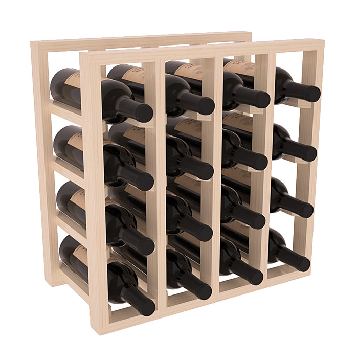 ] .pull-right[ 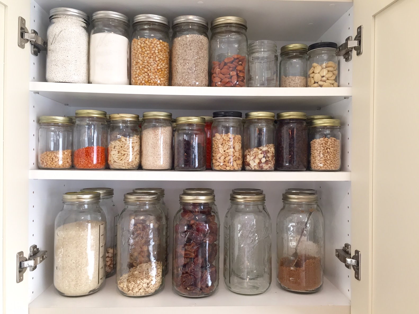 ] --- # Accessing elements from containers You can use the **[]** operator after the name of an object to extract indvidual elements from that object. .pull-left[ ```r one_to_four ``` ``` ## Monday Tuesday Wednesday Thursday ## 1 2 3 4 ``` ```r test_matrix ``` ``` ## [,1] [,2] [,3] ## [1,] 1.3929560 0.2605482 1.3941402 ## [2,] -0.8899093 -0.9559970 -0.2115673 ## [3,] 1.3994929 0.7738423 -0.5347060 ``` ] .pull-right[ ```r one_to_four["Wednesday"] ``` ``` ## Wednesday ## 3 ``` ```r test_matrix[2:3, 1:2] ``` ``` ## [,1] [,2] ## [1,] -0.8899093 -0.9559970 ## [2,] 1.3994929 0.7738423 ``` ] --- background-image: url(images/03/tidy-hex.png) background-position: 50% 75% background-size: 50% class: inverse, middle, center --- background-image: url(images/03/tidy-hex.png) background-position: 90% 5% background-size: 8% # Tidyverse .large[ The **tidyverse** is a collection of packages that expand R's functions in a structured, coherent way. ```r install.packages("tidyverse") ``` ] .large[ There are eight core **tidyverse** packages loaded using **library(tidyverse)**. .pull-left[ * ggplot2 * **tidyr** * dplyr * **tibble** ] .pull-right[ * purrr * readr * stringr * forcats ] ] --- background-image: url(images/03/tidy-hex.png) background-position: 90% 5% background-size: 8% # Tidyverse .large[ You can load all these packages at once. ] ```r library(tidyverse) # This loads all the tidyverse packages at once ``` .large[ You can also load each one individually. We'll be using the **tibble** package next. ] ```r library(tibble) ``` .large[Many of the *tidyverse* packages create or output *tibbles*, which are essentially a more user-friendly version of data frames.] --- # Tibbles You can create a *tibble* similar to how you create a data frame, using **tibble()**. ```r age_tibb <- tibble(Participant = 1:10, cond1 = rnorm(10), age_group = rep(c("Old", "Young"), each = 5)) head(age_tibb) ``` ``` ## # A tibble: 6 x 3 ## Participant cond1 age_group ## <int> <dbl> <chr> ## 1 1 0.653 Old ## 2 2 0.459 Old ## 3 3 1.30 Old ## 4 4 -0.776 Old ## 5 5 -1.64 Old ## 6 6 0.417 Young ``` --- # Tibbles ```r age_tibb <- tibble(Participant = 1:10, cond1 = rnorm(10), * age_group = rep(c("Old", "Young"), each = 5)) ``` Here I used the **rep()** function to generate a character vector with the values "Old" and "Young". ```r rep(c("Old", "Young"), each = 5) ``` ``` ## [1] "Old" "Old" "Old" "Old" "Old" "Young" "Young" "Young" "Young" "Young" ``` ```r rep(c("Old", "Young"), 5) ``` ``` ## [1] "Old" "Young" "Old" "Young" "Old" "Young" "Old" "Young" "Old" "Young" ``` --- class: inverse, center, middle # Relating data to structure --- # Let's think about an *experiment* .large[ The experiment is a reaction time experiment with a two-by-two repeated measures design. Participants see pictures of objects twice. Sometimes they are seen from the *same* viewpoint twice, sometimes from *different* viewpoints each time. There are two separate blocks of trials. The dependent variable is how long it takes them to name the objects, or *reaction time*. You're interested in whether: 1. they get faster at naming object the second time 2. they are faster when the same view is presented both times. ] --- # How many variables are there? |Variables| R Data Type| |--------------|------------| |Participant ID|Numeric or character| |Reaction times|Numeric| |Block first/second|Character/factor| |Viewpoint same/different|Character/factor| .large[ The final dataset needs to be able to do several things. 1. It needs to uniquely identify each participant. 2. It needs to tie each value to the right participant. 3. It needs to identify what each value represents in terms of the design. ] --- class: inverse, center, middle # The many ways to structure data --- # One column for condition, one column for RT .pull-left[ ``` ## # A tibble: 40 x 3 ## # Groups: Participant [10] ## Participant exp_condition RT ## <int> <chr> <dbl> ## 1 1 Block1_different 407. ## 2 1 Block1_same 415. ## 3 1 Block2_different 382. ## 4 1 Block2_same 371. ## 5 2 Block1_different 420. ## 6 2 Block1_same 384. ## 7 2 Block2_different 479. ## 8 2 Block2_same 402. ## 9 3 Block1_different 368. ## 10 3 Block1_same 341. ## # ... with 30 more rows ``` ] .pull-right[ .large[ This is a little awkward. At first glance, there's no easy way to see how many variables there. ] ] --- # Dependent variable split across columns .pull-left[ ``` ## # A tibble: 16 x 4 ## # Groups: Participant [8] ## Participant Viewpoint B1RT B2RT ## <int> <chr> <dbl> <dbl> ## 1 1 Different 536. 364. ## 2 1 Same 494. 450. ## 3 2 Different 511. 393. ## 4 2 Same 432. 371. ## 5 3 Different 536. 364. ## 6 3 Same 494. 450. ## 7 4 Different 511. 393. ## 8 4 Same 432. 371. ## 9 5 Different 536. 364. ## 10 5 Same 494. 450. ## 11 6 Different 511. 393. ## 12 6 Same 432. 371. ## 13 7 Different 536. 364. ## 14 7 Same 494. 450. ## 15 8 Different 511. 393. ## 16 8 Same 432. 371. ``` ] --- # One column per condition ``` ## # A tibble: 10 x 5 ## Participant Block1_same Block2_same Block1_different Block2_different ## <int> <dbl> <dbl> <dbl> <dbl> ## 1 1 515. 268. 546. 413. ## 2 2 471. 249. 535. 449. ## 3 3 507. 331. 501. 386. ## 4 4 482. 312. 607. 389. ## 5 5 484. 322. 595. 431. ## 6 6 502. 301. 527. 359. ## 7 7 520. 328. 557. 398. ## 8 8 579. 272. 578. 378. ## 9 9 441. 290. 572. 401. ## 10 10 526. 285. 550. 405. ``` .large[ This is also called **wide** format. ] --- # How many *variables* are there? ``` ## # A tibble: 10 x 5 ## Participant Block1_same Block2_same Block1_different Block2_different ## <int> <dbl> <dbl> <dbl> <dbl> ## 1 1 515. 268. 546. 413. ## 2 2 471. 249. 535. 449. ## 3 3 507. 331. 501. 386. ## 4 4 482. 312. 607. 389. ## 5 5 484. 322. 595. 431. ## 6 6 502. 301. 527. 359. ## 7 7 520. 328. 557. 398. ## 8 8 579. 272. 578. 378. ## 9 9 441. 290. 572. 401. ## 10 10 526. 285. 550. 405. ``` -- Four... but there are five columns. ```r ncol(example_rt_df) ``` ``` ## [1] 5 ``` --- # How many *observations* are there? ``` ## # A tibble: 10 x 5 ## Participant Block1_same Block2_same Block1_different Block2_different ## <int> <dbl> <dbl> <dbl> <dbl> ## 1 1 515. 268. 546. 413. ## 2 2 471. 249. 535. 449. ## 3 3 507. 331. 501. 386. ## 4 4 482. 312. 607. 389. ## 5 5 484. 322. 595. 431. ## 6 6 502. 301. 527. 359. ## 7 7 520. 328. 557. 398. ## 8 8 579. 272. 578. 378. ## 9 9 441. 290. 572. 401. ## 10 10 526. 285. 550. 405. ``` -- 40... but there are 10 rows. ```r nrow(example_rt_df) ``` ``` ## [1] 10 ``` --- # Your target Switch to *RStudio.cloud* and create a *New Project*. Your job is to try to recreate this *tibble*. ``` ## # A tibble: 10 x 5 ## Participant Block1_same Block2_same Block1_different Block2_different ## <int> <dbl> <dbl> <dbl> <dbl> ## 1 1 508. 340. 522. 295. ## 2 2 523. 268. 550. 470. ## 3 3 543. 303. 667. 476. ## 4 4 556. 408. 400. 322. ## 5 5 506. 163. 539. 269. ## 6 6 489. 287. 350. 363. ## 7 7 398. 346. 624. 392. ## 8 8 470. 494. 504. 374. ## 9 9 517. 258. 396. 422. ## 10 10 642. 348. 515. 437. ``` --- # A shortcut to more tips .large[ If you follow this link, you should be able to make a copy of a project I prepared for you. This project has only one file, an RMarkdown file that has some more tips and instructions for you. https://rstudio.cloud/project/1817564 (if you get really stuck, there is a solution to Part 1 on the next slide!) ] --- # A possible solution ```r set.seed(200) # if you want these exact numbers, use this line example_rt_df <- tibble(Participant = seq(1, 10), Block1_same = rnorm(10, 500, 100), Block2_same = rnorm(10, 350, 100), Block1_different = rnorm(10, 500, 100), Block2_different = rnorm(10, 400, 100)) ``` ``` ## # A tibble: 5 x 5 ## Participant Block1_same Block2_same Block1_different Block2_different ## <int> <dbl> <dbl> <dbl> <dbl> ## 1 1 508. 340. 522. 295. ## 2 2 523. 268. 550. 470. ## 3 3 543. 303. 667. 476. ## 4 4 556. 408. 400. 322. ## 5 5 506. 163. 539. 269. ``` --- class: inverse, center, middle # Tidy data --- background-image: url(images/03/tidy-1.png) background-position: 50% 72% background-size: 75% # The three principles of tidy data 1. Each variable must have its own column. 2. Each observation must have its own row. 3. Each value must have its own cell. --- background-image: url(images/03/tidy-1.png) background-position: 50% 85% background-size: 70% # Why Tidy? .large[ 1. Many functions in R operate on so-called *long* format data, requiring dependent and independent variables to be in different columns of a data frame. 2. Having a consistent way to store and structure your data makes it more *generic*. This makes it easier to use it with different functions. 3. Being *generic* also makes it easier to understand a new dataset in this format. ] --- # One column per condition ``` ## # A tibble: 10 x 5 ## Participant Block1_same Block2_same Block1_different Block2_different ## <int> <dbl> <dbl> <dbl> <dbl> ## 1 1 515. 268. 546. 413. ## 2 2 471. 249. 535. 449. ## 3 3 507. 331. 501. 386. ## 4 4 482. 312. 607. 389. ## 5 5 484. 322. 595. 431. ## 6 6 502. 301. 527. 359. ## 7 7 520. 328. 557. 398. ## 8 8 579. 272. 578. 378. ## 9 9 441. 290. 572. 401. ## 10 10 526. 285. 550. 405. ``` This is also called **wide** format. --- background-image: url(images/03/tidy-7.png) background-position: 50% 78% background-size: 60% # This data is *untidy* .large[ One variable - RT - is split across four columns. Another variable - Block - is split across two columns. A third variable - viewpoint - is also split across two columns. ] --- class: inverse, middle, center # Tidying your data --- # Tidyr The **tidyr** package contains functions to help tidy up your data. We'll look now at **pivot_longer()** and **pivot_wider()**. To start tidying our data, we need the RTs to be in a single column. ```r head(example_rt_df, n = 4) ``` ``` ## # A tibble: 4 x 5 ## Participant Block1_same Block2_same Block1_different Block2_different ## <int> <dbl> <dbl> <dbl> <dbl> ## 1 1 508. 340. 522. 295. ## 2 2 523. 268. 550. 470. ## 3 3 543. 303. 667. 476. ## 4 4 556. 408. 400. 322. ``` The function **pivot_longer()** can be used to combine columns into one. Look at the help using **?pivot_longer** --- # Pivoting longer .pull-left[ ```r pivot_longer(data, cols, names_to = "key", values_to = "value", ...) ``` ] .pull-right[ The first argument, *data*, is the name of the data frame you want to modify. *cols* are the columns you want to combine together. *names_to* is the name of the new column that will contain the values of a single categorical variable. *values_to* is the name of the new column containing the values for each level of that variable. ] --- # Pivoting longer ```r long_rt <- pivot_longer(example_rt_df, cols = c("Block1_same", "Block1_different", "Block2_same", "Block2_different"), names_to = "exp_cond", values_to = "RT") head(long_rt) ``` ``` ## # A tibble: 6 x 3 ## Participant exp_cond RT ## <int> <chr> <dbl> ## 1 1 Block1_same 508. ## 2 1 Block1_different 522. ## 3 1 Block2_same 340. ## 4 1 Block2_different 295. ## 5 2 Block1_same 523. ## 6 2 Block1_different 550. ``` --- # Pivoting longer After we specify the "key" and "value" columns, we need to specify which columns we want to be *gathered*. .pull-left[ ```r long_rt <- pivot_longer(example_rt_df, names_to = "exp_cond", values_to = "RT", cols = 2:5) # here I use numbers head(long_rt) ``` ``` ## # A tibble: 6 x 3 ## Participant exp_cond RT ## <int> <chr> <dbl> ## 1 1 Block1_same 508. ## 2 1 Block2_same 340. ## 3 1 Block1_different 522. ## 4 1 Block2_different 295. ## 5 2 Block1_same 523. ## 6 2 Block2_same 268. ``` ] .pull-right[ ```r long_rt <- pivot_longer(example_rt_df, names_to = "exp_cond", values_to = "RT", cols = Block1_same:Block2_different) # here I use names head(long_rt) ``` ``` ## # A tibble: 6 x 3 ## Participant exp_cond RT ## <int> <chr> <dbl> ## 1 1 Block1_same 508. ## 2 1 Block2_same 340. ## 3 1 Block1_different 522. ## 4 1 Block2_different 295. ## 5 2 Block1_same 523. ## 6 2 Block2_same 268. ``` ] --- # Splitting columns We have the RTs in one column, but we still have another problem: The "Block" and "Viewpoint" variables are combined into a single column. ```r head(long_rt) ``` ``` ## # A tibble: 6 x 3 ## Participant exp_cond RT ## <int> <chr> <dbl> ## 1 1 Block1_same 508. ## 2 1 Block2_same 340. ## 3 1 Block1_different 522. ## 4 1 Block2_different 295. ## 5 2 Block1_same 523. ## 6 2 Block2_same 268. ``` --- # Splitting columns Fortunately, the values in the *exp_cond* column can be easily split: ```r unique(long_rt$exp_cond) ``` ``` ## [1] "Block1_same" "Block2_same" "Block1_different" "Block2_different" ``` The value of "Block" comes before the underscore ("_"), while the value of "viewpoint" comes after it. --- # Splitting columns ```r long_rt <- pivot_longer(example_rt_df, names_to = c("Block", "Viewpoint"), names_sep = "_", values_to = "RT", cols = Block1_same:Block2_different) head(long_rt) ``` ``` ## # A tibble: 6 x 4 ## Participant Block Viewpoint RT ## <int> <chr> <chr> <dbl> ## 1 1 Block1 same 508. ## 2 1 Block2 same 340. ## 3 1 Block1 different 522. ## 4 1 Block2 different 295. ## 5 2 Block1 same 523. ## 6 2 Block2 same 268. ``` --- # Splitting columns Let's look at the additional syntax. ```r pivot_longer(example_rt_df, names_to = c("Block", "Viewpoint"), names_sep = "_", values_to = "RT", cols = Block1_same:Block2_different) ``` `names_to` now has two entries, one for each new column that will be made. `names_sep` is the character that *separates* the values you want to split. --- # Your target .pull-left[ ``` ## # A tibble: 15 x 4 ## Participant Block Viewpoint RT ## <int> <chr> <chr> <dbl> ## 1 1 Block1 same 508. ## 2 1 Block2 same 340. ## 3 1 Block1 different 522. ## 4 1 Block2 different 295. ## 5 2 Block1 same 523. ## 6 2 Block2 same 268. ## 7 2 Block1 different 550. ## 8 2 Block2 different 470. ## 9 3 Block1 same 543. ## 10 3 Block2 same 303. ## 11 3 Block1 different 667. ## 12 3 Block2 different 476. ## 13 4 Block1 same 556. ## 14 4 Block2 same 408. ## 15 4 Block1 different 400. ``` ] .pull-right[ You should specify name(s) for the column(s) that you'll create using the "names_to" and "values_to" arguments. You'll need to add "names_sep" and the character that separates the two sides as well in order to match the target ] --- class: inverse, center, middle # Pivoting wider --- # Pivoting wider Sometimes you want to go in the *opposite* direction. **pivot_wider()** is the *opposite* of **pivot_longer()**. ```r wide_rt <- pivot_wider(long_rt, names_from = c("Block", "Viewpoint"), values_from = "RT") head(wide_rt, 10) ``` ``` ## # A tibble: 10 x 5 ## Participant Block1_same Block2_same Block1_different Block2_different ## <int> <dbl> <dbl> <dbl> <dbl> ## 1 1 508. 340. 522. 295. ## 2 2 523. 268. 550. 470. ## 3 3 543. 303. 667. 476. ## 4 4 556. 408. 400. 322. ## 5 5 506. 163. 539. 269. ## 6 6 489. 287. 350. 363. ## 7 7 398. 346. 624. 392. ## 8 8 470. 494. 504. 374. ## 9 9 517. 258. 396. 422. ## 10 10 642. 348. 515. 437. ``` --- class: inverse, middle, center # Now what? --- # Now that it's tidy... Now that we've got the data in a tidy format, we can begin to use some of the more interesting features of R! We can produce a boxplot using **ggplot2** (more next week!) .pull-left[ 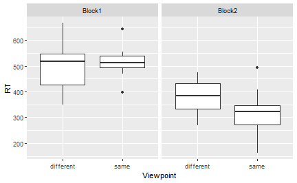<!-- --> ] .pull-right[ 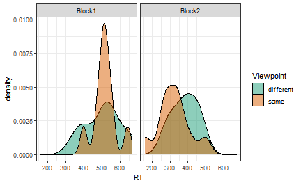<!-- --> ] --- # Now that it's tidy... We can produce some summary statistics using **dplyr** (more soon!) ``` ## `summarise()` regrouping output by 'Block' (override with `.groups` argument) ``` ``` ## # A tibble: 4 x 4 ## # Groups: Block [2] ## Block Viewpoint mean_RT sd_RT ## <chr> <chr> <dbl> <dbl> ## 1 Block1 different 507. 100. ## 2 Block1 same 515. 62.5 ## 3 Block2 different 382. 71.2 ## 4 Block2 same 321. 89.7 ``` --- # Now that it's tidy... We can run ANOVA with **afex**. ``` ## Anova Table (Type 3 tests) ## ## Response: RT ## Effect df MSE F ges p.value ## 1 Block 1, 9 5222.72 48.56 *** .510 <.001 ## 2 Viewpoint 1, 9 7794.41 0.87 .027 .376 ## 3 Block:Viewpoint 1, 9 6343.29 1.87 .046 .205 ## --- ## Signif. codes: 0 '***' 0.001 '**' 0.01 '*' 0.05 '+' 0.1 ' ' 1 ``` --- # Now that it's tidy... We can create interaction plots using **emmeans**. .pull-left[ <!-- --> ] .pull-right[ ``` ## Block = Block1: ## contrast estimate SE df t.ratio p.value ## same - different 8.43 37.6 17.8 0.224 0.8251 ## ## Block = Block2: ## contrast estimate SE df t.ratio p.value ## same - different -60.45 37.6 17.8 -1.608 0.1255 ``` ] --- # Next week .large[ - The following chapters of R for Data Science - - **Data Visualization** (Chapter 1 via the library) - **Graphics for communication with ggplot2** (Chapter 22 via the library) Practice some of the skills for next week: - **RStudio.cloud Primer** - Visualize Data ]