Importing, transforming, and summarising your data

class: center, middle, inverse, title-slide

# Importing, transforming, and summarising your data
### 10/11/2020

---

# Plotting using ggplot2

.pull-left[

```r
ggplot(data = mpg, 
       mapping = aes(x = displ,
                     y = hwy,
                     colour = factor(cyl))) +
  geom_point() + 
  geom_smooth(method = "lm", se = FALSE) + 
  labs(x = "Engine displacement (litres)",
       y = "Highway miles per gallon",
       colour = "Cylinders")
```

```
## `geom_smooth()` using formula 'y ~ x'
```
]
.pull-right[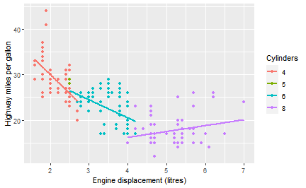
![](Week-5-Import-and-wrangling_files/figure-html/scatter-cyls-smo-1.png)
]

---
class: center, middle, inverse
# A quick reminder

.large[
For anyone that hasn't done this already, join the PSY9219M workspace on RStudio.cloud.

# https://bit.ly/PSYWorkspace
]

---
class: middle, center, inverse
# Importing your data

---
# Different types of file

Data comes in many different shapes, sizes, and formats.

The most common file formats you'll deal with are either Excel files or text files, but you may also find dealing with SPSS files useful.

Fortunately, R has several functions and packages for importing data!

---
# Importing data into R

.pull-left[
## Comma-separated values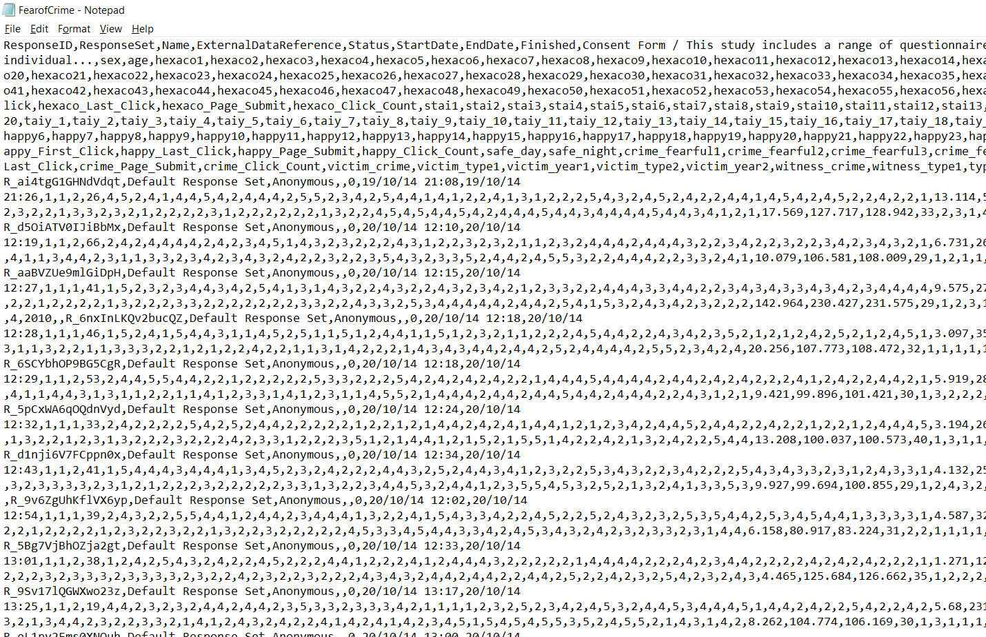
![:scale 90%](images/05/foc_csv.png)
]
.pull-right[
## Excel spreadsheets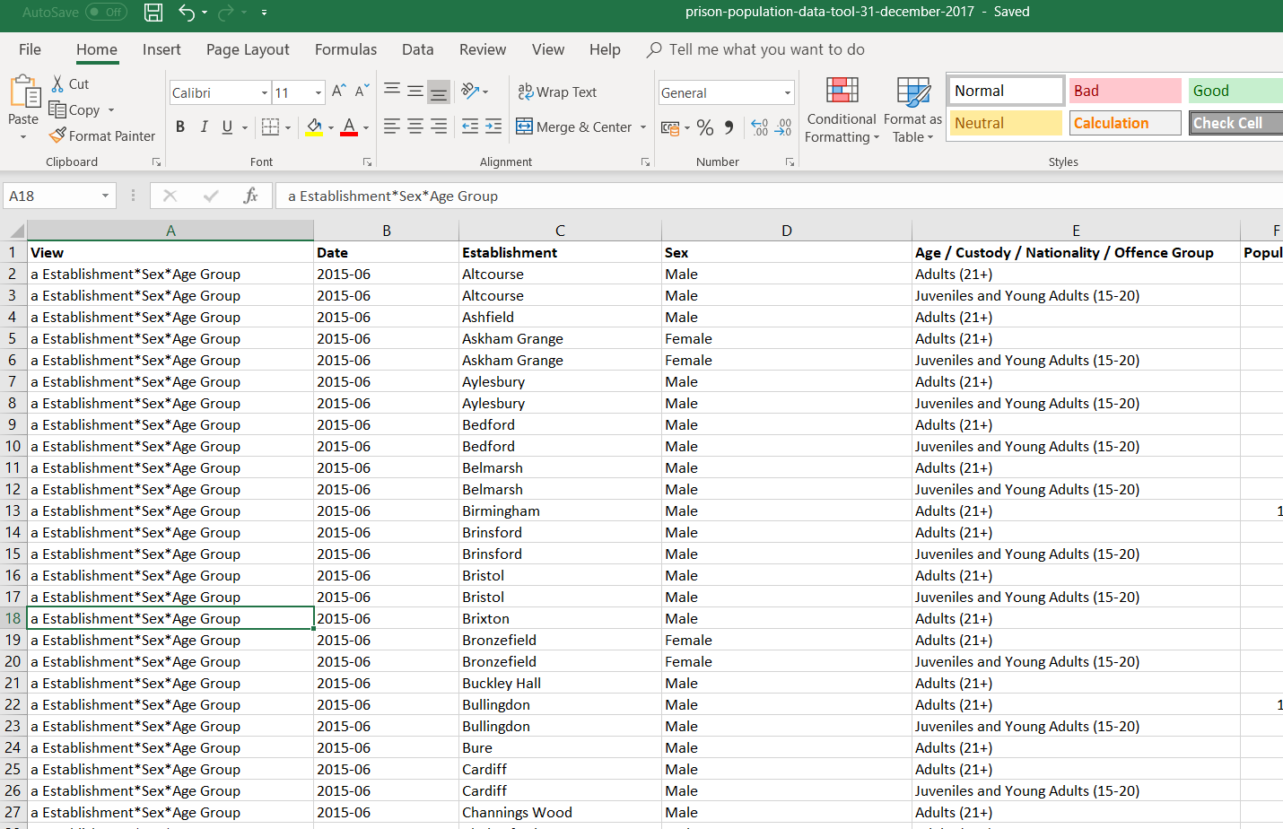
![:scale 90%](images/05/excel_style.png)
]

---
# Fear of Crime Dataset

[Ellis & Renouf (2018)](https://doi.org/10.1080/14789949.2017.1410562) - the relationship between fear of crime and various personality measures.

Their data is openly available, stored as text in a *comma-separated-values* format (*.csv*).

Once again, we can use the import button or some code (with **read_csv()**) to load this data in and automatically format it into a *tibble*.

```r
library(readr)
FearofCrime <- read_csv("data/FearofCrime.CSV")
```

See also [Ellis & Merdian, 2015](https://doi.org/10.3389/fpsyg.2015.01782), Frontiers in Psychology
---
# Fear of Crime Dataset

Ellis & Renouf (2018) collected data online using Qualtrics.

The file contains one column for each question that the participants answered, for a total of 169(!) columns.

Each row is a single participant's answers, and their demographic information.

```r
FearofCrime
```

```
## # A tibble: 301 x 169
##    ResponseID ResponseSet Name  ExternalDataRef~ Status StartDate EndDate Finished `Consent Form /~   sex   age
##    <chr>      <chr>       <chr> <lgl>             <dbl> <chr>     <chr>      <dbl>            <dbl> <dbl> <dbl>
##  1 R_ai4tgG1~ Default Re~ Anon~ NA                    0 19/10/14~ 19/10/~        1                1     2    26
##  2 R_d5OiATV~ Default Re~ Anon~ NA                    0 20/10/14~ 20/10/~        1                1     2    66
##  3 R_aaBVZUe~ Default Re~ Anon~ NA                    0 20/10/14~ 20/10/~        1                1     1    41
##  4 R_6nxInLK~ Default Re~ Anon~ NA                    0 20/10/14~ 20/10/~        1                1     1    46
##  5 R_6SCYbhO~ Default Re~ Anon~ NA                    0 20/10/14~ 20/10/~        1                1     2    53
##  6 R_5pCxWA6~ Default Re~ Anon~ NA                    0 20/10/14~ 20/10/~        1                1     1    33
##  7 R_d1nji6V~ Default Re~ Anon~ NA                    0 20/10/14~ 20/10/~        1                1     2    41
##  8 R_9v6ZgUh~ Default Re~ Anon~ NA                    0 20/10/14~ 20/10/~        1                1     1    39
##  9 R_5Bg7VjB~ Default Re~ Anon~ NA                    0 20/10/14~ 20/10/~        1                1     2    38
## 10 R_9Sv17lQ~ Default Re~ Anon~ NA                    0 20/10/14~ 20/10/~        1                1     2    19
## # ... with 291 more rows, and 158 more variables: hexaco1 <dbl>, hexaco2 <dbl>, hexaco3 <dbl>, hexaco4 <dbl>,
## #   hexaco5 <dbl>, hexaco6 <dbl>, hexaco7 <dbl>, hexaco8 <dbl>, hexaco9 <dbl>, hexaco10 <dbl>, hexaco11 <dbl>,
## #   hexaco12 <dbl>, hexaco13 <dbl>, hexaco14 <dbl>, hexaco15 <dbl>, hexaco16 <dbl>, hexaco17 <dbl>,
## #   hexaco18 <dbl>, hexaco19 <dbl>, hexaco20 <dbl>, hexaco21 <dbl>, hexaco22 <dbl>, hexaco23 <dbl>,
## #   hexaco24 <dbl>, hexaco25 <dbl>, hexaco26 <dbl>, hexaco27 <dbl>, hexaco28 <dbl>, hexaco29 <dbl>,
## #   hexaco30 <dbl>, hexaco31 <dbl>, hexaco32 <dbl>, hexaco33 <dbl>, hexaco34 <dbl>, hexaco35 <dbl>,
## #   hexaco36 <dbl>, hexaco37 <dbl>, hexaco38 <dbl>, hexaco39 <dbl>, hexaco40 <dbl>, hexaco41 <dbl>,
## #   hexaco42 <dbl>, hexaco43 <dbl>, hexaco44 <dbl>, hexaco45 <dbl>, hexaco46 <dbl>, hexaco47 <dbl>,
## #   hexaco48 <dbl>, hexaco49 <dbl>, hexaco50 <dbl>, hexaco51 <dbl>, hexaco52 <dbl>, hexaco53 <dbl>,
## #   hexaco54 <dbl>, hexaco55 <dbl>, hexaco56 <dbl>, hexaco57 <dbl>, hexaco58 <dbl>, hexaco59 <dbl>,
## #   hexaco60 <dbl>, hexaco_First_Click <dbl>, hexaco_Last_Click <dbl>, hexaco_Page_Submit <dbl>,
## #   hexaco_Click_Count <dbl>, stai1 <dbl>, stai2 <dbl>, stai3 <dbl>, stai4 <dbl>, stai5 <dbl>, stai6 <dbl>,
## #   stai7 <dbl>, stai8 <dbl>, stai9 <dbl>, stai10 <dbl>, stai11 <dbl>, stai12 <dbl>, stai13 <dbl>,
## #   stai14 <dbl>, stai15 <dbl>, stai16 <dbl>, stai17 <dbl>, stai18 <dbl>, stai19 <dbl>, stai20 <dbl>,
## #   taiy_1 <dbl>, taiy_2 <dbl>, taiy_3 <dbl>, taiy_4 <dbl>, taiy_5 <dbl>, taiy_6 <dbl>, taiy_7 <dbl>,
## #   taiy_8 <dbl>, taiy_9 <dbl>, taiy_10 <dbl>, taiy_11 <dbl>, taiy_12 <dbl>, taiy_13 <dbl>, taiy_14 <dbl>,
## #   taiy_15 <dbl>, taiy_16 <dbl>, ...
```

---
background-image: url(images/05/import-data-button.png)
background-size: contain
class: inverse

---
background-image: url(images/05/import-text-dialog.png)
background-size: contain
class: inverse

---
background-image: url(images/05/import-text-browse.png)
background-size: contain
class: inverse

---
background-image: url(images/05/import-text-url.png)
background-size: contain
class: inverse

---
background-image: url(images/05/import-text-code-prev.png)
background-size: contain
class: inverse

---
background-image: url(images/05/import-foc.png)
background-size: contain
class: inverse

---
# Prison population

Last week, we looked at some data regarding the UK's prison population.

The data is contained in an [Excel spreadsheet](https://assets.publishing.service.gov.uk/government/uploads/system/uploads/attachment_data/file/676248/prison-population-data-tool-31-december-2017.xlsx), downloaded from [data.gov.uk](https://data.gov.uk).

```r
library(readxl)
prison_pop <- read_excel("data/prison-population-data-tool-31-december-2017.xlsx",
                         sheet = "PT Data")
```

We use the **read_excel()** function to read Excel files.

Note how the file name and location come first, and then I specify a specific *sheet*.

Excel spreadsheets often have multiple sheets with different information.

---
background-image: url(images/05/import-from-excel.png)
background-size: contain
class: inverse

---
background-image: url(images/05/import-from-excel-change.png)
background-size: contain
class: inverse

---
background-image: url(images/05/import-from-excel-changed.png)
background-size: contain
class: inverse

---
# Prison population

Once the data is imported, we have a *tibble*.

We can immediately see there are 6 columns with 22409 rows.

```r
prison_pop
```

```
## # A tibble: 22,409 x 6
##    View                       Date    Establishment Sex    `Age / Custody / Nationality / Offence G~ Population
##    <chr>                      <chr>   <chr>         <chr>  <chr>                                          <dbl>
##  1 a Establishment*Sex*Age G~ 2015-06 Altcourse     Male   Adults (21+)                                     922
##  2 a Establishment*Sex*Age G~ 2015-06 Altcourse     Male   Juveniles and Young Adults (15-20)               169
##  3 a Establishment*Sex*Age G~ 2015-06 Ashfield      Male   Adults (21+)                                     389
##  4 a Establishment*Sex*Age G~ 2015-06 Askham Grange Female Adults (21+)                                      NA
##  5 a Establishment*Sex*Age G~ 2015-06 Askham Grange Female Juveniles and Young Adults (15-20)                NA
##  6 a Establishment*Sex*Age G~ 2015-06 Aylesbury     Male   Adults (21+)                                     113
##  7 a Establishment*Sex*Age G~ 2015-06 Aylesbury     Male   Juveniles and Young Adults (15-20)               268
##  8 a Establishment*Sex*Age G~ 2015-06 Bedford       Male   Adults (21+)                                     459
##  9 a Establishment*Sex*Age G~ 2015-06 Bedford       Male   Juveniles and Young Adults (15-20)                30
## 10 a Establishment*Sex*Age G~ 2015-06 Belmarsh      Male   Adults (21+)                                     794
## # ... with 22,399 more rows
```

We need to do more work to make this file useable...

---
background-image: url(images/05/dplyr-logo.png)
background-size: 6%
background-position: 50% 75%
class: middle, center, inverse
# dpylr and data transformation

---
background-image: url(images/05/dplyr-logo.png)
background-size: 6%
background-position: 90% 5%
# Data transformation

With datasets like those we've loaded, there are often organisational issues.

For example, there could be many columns or rows we don't need, or the data would make more sense if it were sorted.

This is where **dplyr** comes in!

|Function |Effect|
|------------|----|
| select()   |Include or exclude variables (columns)|
| arrange()  |Change the order of observations (rows)|
| filter()   |Include or exclude observations (rows)|
| mutate()   |Create new variables (columns)|
| group_by() |Create groups of observations|
| summarise()|Aggregate or summarise groups of observations (rows)|

---
class: inverse, middle, center
# Selecting columns

---
background-image: url(images/05/dplyr-logo.png)
background-size: 6%
background-position: 90% 5%
# Selecting columns

.large[
Sometimes only some columns are of interest.

The Fear of Crime dataset has 169 columns. Only some of them are useful; here are the first ten.
]

```r
names(FearofCrime)[1:10]
```

```
##  [1] "ResponseID"                                                                                             
##  [2] "ResponseSet"                                                                                            
##  [3] "Name"                                                                                                   
##  [4] "ExternalDataReference"                                                                                  
##  [5] "Status"                                                                                                 
##  [6] "StartDate"                                                                                              
##  [7] "EndDate"                                                                                                
##  [8] "Finished"                                                                                               
##  [9] "Consent Form / This study includes a range of questionnaires collecting / demographic and individual..."
## [10] "sex"
```

---
background-image: url(images/05/dplyr-logo.png)
background-size: 6%
background-position: 90% 5%

# Selecting columns

.pull-left[
.large[
We pass the name of the data frame that we want to select from, and the names of each column we want to keep after that.

Suppose that, first of all, we were only interested in the age and sex of our participants.
]
]
.pull-right[

```r
select(FearofCrime, age, sex)
```

```
## # A tibble: 301 x 2
##      age   sex
##    <dbl> <dbl>
##  1    26     2
##  2    66     2
##  3    41     1
##  4    46     1
##  5    53     2
##  6    33     1
##  7    41     2
##  8    39     1
##  9    38     2
## 10    19     2
## # ... with 291 more rows
```
]

---
background-image: url(images/05/dplyr-logo.png)
background-size: 6%
background-position: 90% 5%

# Selecting columns

.pull-left[
.large[
The HEXACO-PI-R is a personality questionnaire that aims to measure six factors - Honesty-Humility, Emotionality, Extraversion, Agreeableness, Conscientiousness, and Openness to Experience.

The Fear of Crime dataset has the participants answers to the 60 questions of the HEXACO-PI-R in 60 columns. 
]
]
.pull-right[

```r
select(FearofCrime, hexaco1,
       hexaco2, hexaco3)
```

```
## # A tibble: 8 x 3
##   hexaco1 hexaco2 hexaco3
##     <dbl>   <dbl>   <dbl>
## 1       4       5       2
## 2       2       4       2
## 3       1       5       2
## 4       1       5       2
## 5       2       4       4
## 6       2       4       2
## 7       1       5       4
## 8       2       4       3
```
]

---
background-image: url(images/05/dplyr-logo.png)
background-size: 6%
background-position: 90% 5%
# Selecting columns

Typing these out one by one would be ... *laborious*.

Fortunately, there are some shorthands.

The colon (*:*) operator can be used to say "everything between these columns (inclusive)".

```r
select(FearofCrime, hexaco1:hexaco5)
```

```
## # A tibble: 301 x 5
##    hexaco1 hexaco2 hexaco3 hexaco4 hexaco5
##      <dbl>   <dbl>   <dbl>   <dbl>   <dbl>
##  1       4       5       2       4       1
##  2       2       4       2       4       4
##  3       1       5       2       3       2
##  4       1       5       2       4       1
##  5       2       4       4       5       5
##  6       2       4       2       2       2
##  7       1       5       4       4       4
##  8       2       4       3       2       2
##  9       1       2       4       2       5
## 10       4       4       2       3       2
## # ... with 291 more rows
```

---
background-image: url(images/05/dplyr-logo.png)
background-size: 6%
background-position: 90% 5%

# Selecting columns
.large[
Note that you can also tell **select()** to *remove* columns using the minus (*-*) sign.
]

```r
head(FearofCrime, 6)
```

```
## # A tibble: 6 x 169
##   ResponseID ResponseSet Name  ExternalDataRef~ Status StartDate EndDate Finished `Consent Form /~   sex   age
##   <chr>      <chr>       <chr> <lgl>             <dbl> <chr>     <chr>      <dbl>            <dbl> <dbl> <dbl>
## 1 R_ai4tgG1~ Default Re~ Anon~ NA                    0 19/10/14~ 19/10/~        1                1     2    26
## 2 R_d5OiATV~ Default Re~ Anon~ NA                    0 20/10/14~ 20/10/~        1                1     2    66
## 3 R_aaBVZUe~ Default Re~ Anon~ NA                    0 20/10/14~ 20/10/~        1                1     1    41
## 4 R_6nxInLK~ Default Re~ Anon~ NA                    0 20/10/14~ 20/10/~        1                1     1    46
## 5 R_6SCYbhO~ Default Re~ Anon~ NA                    0 20/10/14~ 20/10/~        1                1     2    53
## 6 R_5pCxWA6~ Default Re~ Anon~ NA                    0 20/10/14~ 20/10/~        1                1     1    33
## # ... with 158 more variables: hexaco1 <dbl>, hexaco2 <dbl>, hexaco3 <dbl>, hexaco4 <dbl>, hexaco5 <dbl>,
## #   hexaco6 <dbl>, hexaco7 <dbl>, hexaco8 <dbl>, hexaco9 <dbl>, hexaco10 <dbl>, hexaco11 <dbl>,
## #   hexaco12 <dbl>, hexaco13 <dbl>, hexaco14 <dbl>, hexaco15 <dbl>, hexaco16 <dbl>, hexaco17 <dbl>,
## #   hexaco18 <dbl>, hexaco19 <dbl>, hexaco20 <dbl>, hexaco21 <dbl>, hexaco22 <dbl>, hexaco23 <dbl>,
## #   hexaco24 <dbl>, hexaco25 <dbl>, hexaco26 <dbl>, hexaco27 <dbl>, hexaco28 <dbl>, hexaco29 <dbl>,
## #   hexaco30 <dbl>, hexaco31 <dbl>, hexaco32 <dbl>, hexaco33 <dbl>, hexaco34 <dbl>, hexaco35 <dbl>,
## #   hexaco36 <dbl>, hexaco37 <dbl>, hexaco38 <dbl>, hexaco39 <dbl>, hexaco40 <dbl>, hexaco41 <dbl>,
## #   hexaco42 <dbl>, hexaco43 <dbl>, hexaco44 <dbl>, hexaco45 <dbl>, hexaco46 <dbl>, hexaco47 <dbl>,
## #   hexaco48 <dbl>, hexaco49 <dbl>, hexaco50 <dbl>, hexaco51 <dbl>, hexaco52 <dbl>, hexaco53 <dbl>,
## #   hexaco54 <dbl>, hexaco55 <dbl>, hexaco56 <dbl>, hexaco57 <dbl>, hexaco58 <dbl>, hexaco59 <dbl>,
## #   hexaco60 <dbl>, hexaco_First_Click <dbl>, hexaco_Last_Click <dbl>, hexaco_Page_Submit <dbl>,
## #   hexaco_Click_Count <dbl>, stai1 <dbl>, stai2 <dbl>, stai3 <dbl>, stai4 <dbl>, stai5 <dbl>, stai6 <dbl>,
## #   stai7 <dbl>, stai8 <dbl>, stai9 <dbl>, stai10 <dbl>, stai11 <dbl>, stai12 <dbl>, stai13 <dbl>,
## #   stai14 <dbl>, stai15 <dbl>, stai16 <dbl>, stai17 <dbl>, stai18 <dbl>, stai19 <dbl>, stai20 <dbl>,
## #   taiy_1 <dbl>, taiy_2 <dbl>, taiy_3 <dbl>, taiy_4 <dbl>, taiy_5 <dbl>, taiy_6 <dbl>, taiy_7 <dbl>,
## #   taiy_8 <dbl>, taiy_9 <dbl>, taiy_10 <dbl>, taiy_11 <dbl>, taiy_12 <dbl>, taiy_13 <dbl>, taiy_14 <dbl>,
## #   taiy_15 <dbl>, taiy_16 <dbl>, ...
```

---
background-image: url(images/05/dplyr-logo.png)
background-size: 6%
background-position: 90% 5%

# Selecting columns

Here, I remove a few columns that don't contain any useful information.

```r
select(FearofCrime, -ResponseSet, -Name, -Status, -ExternalDataReference)
```

```
## # A tibble: 301 x 165
##    ResponseID StartDate EndDate Finished `Consent Form /~   sex   age hexaco1 hexaco2 hexaco3 hexaco4 hexaco5
##    <chr>      <chr>     <chr>      <dbl>            <dbl> <dbl> <dbl>   <dbl>   <dbl>   <dbl>   <dbl>   <dbl>
##  1 R_ai4tgG1~ 19/10/14~ 19/10/~        1                1     2    26       4       5       2       4       1
##  2 R_d5OiATV~ 20/10/14~ 20/10/~        1                1     2    66       2       4       2       4       4
##  3 R_aaBVZUe~ 20/10/14~ 20/10/~        1                1     1    41       1       5       2       3       2
##  4 R_6nxInLK~ 20/10/14~ 20/10/~        1                1     1    46       1       5       2       4       1
##  5 R_6SCYbhO~ 20/10/14~ 20/10/~        1                1     2    53       2       4       4       5       5
##  6 R_5pCxWA6~ 20/10/14~ 20/10/~        1                1     1    33       2       4       2       2       2
##  7 R_d1nji6V~ 20/10/14~ 20/10/~        1                1     2    41       1       5       4       4       4
##  8 R_9v6ZgUh~ 20/10/14~ 20/10/~        1                1     1    39       2       4       3       2       2
##  9 R_5Bg7VjB~ 20/10/14~ 20/10/~        1                1     2    38       1       2       4       2       5
## 10 R_9Sv17lQ~ 20/10/14~ 20/10/~        1                1     2    19       4       4       2       3       2
## # ... with 291 more rows, and 153 more variables: hexaco6 <dbl>, hexaco7 <dbl>, hexaco8 <dbl>, hexaco9 <dbl>,
## #   hexaco10 <dbl>, hexaco11 <dbl>, hexaco12 <dbl>, hexaco13 <dbl>, hexaco14 <dbl>, hexaco15 <dbl>,
## #   hexaco16 <dbl>, hexaco17 <dbl>, hexaco18 <dbl>, hexaco19 <dbl>, hexaco20 <dbl>, hexaco21 <dbl>,
## #   hexaco22 <dbl>, hexaco23 <dbl>, hexaco24 <dbl>, hexaco25 <dbl>, hexaco26 <dbl>, hexaco27 <dbl>,
## #   hexaco28 <dbl>, hexaco29 <dbl>, hexaco30 <dbl>, hexaco31 <dbl>, hexaco32 <dbl>, hexaco33 <dbl>,
## #   hexaco34 <dbl>, hexaco35 <dbl>, hexaco36 <dbl>, hexaco37 <dbl>, hexaco38 <dbl>, hexaco39 <dbl>,
## #   hexaco40 <dbl>, hexaco41 <dbl>, hexaco42 <dbl>, hexaco43 <dbl>, hexaco44 <dbl>, hexaco45 <dbl>,
## #   hexaco46 <dbl>, hexaco47 <dbl>, hexaco48 <dbl>, hexaco49 <dbl>, hexaco50 <dbl>, hexaco51 <dbl>,
## #   hexaco52 <dbl>, hexaco53 <dbl>, hexaco54 <dbl>, hexaco55 <dbl>, hexaco56 <dbl>, hexaco57 <dbl>,
## #   hexaco58 <dbl>, hexaco59 <dbl>, hexaco60 <dbl>, hexaco_First_Click <dbl>, hexaco_Last_Click <dbl>,
## #   hexaco_Page_Submit <dbl>, hexaco_Click_Count <dbl>, stai1 <dbl>, stai2 <dbl>, stai3 <dbl>, stai4 <dbl>,
## #   stai5 <dbl>, stai6 <dbl>, stai7 <dbl>, stai8 <dbl>, stai9 <dbl>, stai10 <dbl>, stai11 <dbl>, stai12 <dbl>,
## #   stai13 <dbl>, stai14 <dbl>, stai15 <dbl>, stai16 <dbl>, stai17 <dbl>, stai18 <dbl>, stai19 <dbl>,
## #   stai20 <dbl>, taiy_1 <dbl>, taiy_2 <dbl>, taiy_3 <dbl>, taiy_4 <dbl>, taiy_5 <dbl>, taiy_6 <dbl>,
## #   taiy_7 <dbl>, taiy_8 <dbl>, taiy_9 <dbl>, taiy_10 <dbl>, taiy_11 <dbl>, taiy_12 <dbl>, taiy_13 <dbl>,
## #   taiy_14 <dbl>, taiy_15 <dbl>, taiy_16 <dbl>, taiy_17 <dbl>, taiy_18 <dbl>, taiy_19 <dbl>, taiy_20 <dbl>,
## #   happy1 <dbl>, ...
```

---
class: inverse, center, middle
# Creating new columns

---
background-image: url(images/05/dplyr-logo.png)
background-size: 6%
background-position: 90% 5%

# Creating new columns

Here is a version of the Fear of Crime data where participants' overall scores on the various personality measures have been calculated.

```r
crime
```

```
## # A tibble: 301 x 15
##    Participant       sex     age victim_crime     H     E     X     A     C     O    SA    TA   OHQ   FoC  Foc2
##    <chr>             <chr> <dbl> <chr>        <dbl> <dbl> <dbl> <dbl> <dbl> <dbl> <dbl> <dbl> <dbl> <dbl> <dbl>
##  1 R_01TjXgC191rVSst male     55 yes            3.7   3     3.4   3.9   3.2   3.6  1.15  1.55  3.41   2.6     3
##  2 R_0dN5YeULcyms2qN fema~    20 no             2.5   3.1   2.5   2.4   2.2   3.1  2.05  2.95  2.38   2       3
##  3 R_0DPiPYWhncWS1TX male     57 yes            2.6   3.1   3.3   3.1   4.3   2.8  2     2.6   3      1.2     2
##  4 R_0f7bSsH6Up0yelz male     19 no             3.5   1.8   3.3   3.4   2.1   2.7  1.55  2.1   3.48   3.2     5
##  5 R_0rov2RoSkPEOvlv fema~    20 no             3.3   3.4   3.9   3.2   2.8   3.9  1.3   1.8   3.59   2.8     3
##  6 R_0wioqGERxElVTh3 fema~    20 no             2.6   2.6   3     2.6   2.9   3.4  2.55  1.5   3.76   2       4
##  7 R_0wRO8lNe0kusHNX male     34 yes            3.2   2.5   3.2   2.8   4     3.2  1.85  1.75  3.62   1.6     2
##  8 R_116nEdFsGDrKKzs fema~    19 no             2.9   4     3.9   4.2   3.7   1.9  1.1   2     3.55   2       5
##  9 R_11ZmBd5VEkW4525 fema~    19 yes            3.4   3.4   3.3   3.4   3.2   3.2  2.2   2.9   3.41   3.4     6
## 10 R_12i26Qzosmrr1KE male     20 no             2.4   2.1   1.8   2.2   3.4   2.9  2.15  2.4   2.59   1.4     2
## # ... with 291 more rows
```

---
background-image: url(images/05/dplyr-logo.png)
background-size: 6%
background-position: 90% 5%

# Creating new columns

```r
crime_sub <- select(crime,
                    age, SA, TA, sex)
mutate(crime_sub, age_group = ifelse(age > 40,
                                     "Over 40",
                                     "40 or under"))
```

```
## # A tibble: 301 x 5
##      age    SA    TA sex    age_group  
##    <dbl> <dbl> <dbl> <chr>  <chr>      
##  1    55  1.15  1.55 male   Over 40    
##  2    20  2.05  2.95 female 40 or under
##  3    57  2     2.6  male   Over 40    
##  4    19  1.55  2.1  male   40 or under
##  5    20  1.3   1.8  female 40 or under
##  6    20  2.55  1.5  female 40 or under
##  7    34  1.85  1.75 male   40 or under
##  8    19  1.1   2    female 40 or under
##  9    19  2.2   2.9  female 40 or under
## 10    20  2.15  2.4  male   40 or under
## # ... with 291 more rows
```

---
background-image: url(images/05/dplyr-logo.png)
background-size: 6%
background-position: 90% 5%

# Arranging rows

Having calculated each person's *state anxiety* score, perhaps we'd now like to check who has the lowest and highest scores (note: this can be a good way to check for extreme values!).

.pull-left[

```r
arrange(crime_sub, SA)
```

```
## # A tibble: 301 x 4
##      age    SA    TA sex   
##    <dbl> <dbl> <dbl> <chr> 
##  1    20  1     1.05 male  
##  2    53  1     1.55 female
##  3    49  1     1.65 male  
##  4    19  1.05  1.5  female
##  5    19  1.1   2    female
##  6    19  1.1   1.4  male  
##  7    29  1.1   1.5  female
##  8    19  1.1   1.3  female
##  9    20  1.1   1.8  female
## 10    21  1.1   2.1  male  
## # ... with 291 more rows
```
]
.pull-right[

```r
arrange(crime_sub, desc(SA))
```

```
## # A tibble: 301 x 4
##      age    SA    TA sex   
##    <dbl> <dbl> <dbl> <chr> 
##  1    19  3.85  3.85 female
##  2    20  3.6   3.6  female
##  3    20  3.6   3.55 female
##  4    18  3.4   4    female
##  5    19  3.4   3.35 female
##  6    20  3.35  2.8  female
##  7    20  3.3   3.5  male  
##  8    19  3.2   2.95 male  
##  9    19  3.1   3.1  female
## 10    20  3.1   3.15 female
## # ... with 291 more rows
```
]
---
class: inverse, middle, center
# Grouping and summarizing

---
background-image: url(images/05/dplyr-logo.png)
background-size: 6%
background-position: 90% 5%

# Summarising rows

.pull-left[
A common task when analyzing data is to create summaries of statistical characteristics.

Here I calculate the *mean*, *standard deviation*, and *variance* of the State Anxiety variable.

Other possible summmary functions (other than **mean()**, **sd()**, or **var()**) include **max()**, **min()**, **IQR()**, or **median()**.
]
.pull-right[

```r
summarise(crime,
          mean = mean(SA),
          standard_dev = sd(SA),
          variance = var(SA))
```

```
## # A tibble: 1 x 3
##    mean standard_dev variance
##   <dbl>        <dbl>    <dbl>
## 1  1.92        0.554    0.307
```
]

---
background-image: url(images/05/dplyr-logo.png)
background-size: 6%
background-position: 90% 5%

# Grouping observations

**group_by()** is used to organise data frames into groups according to categorical variables.

```r
grouped_crime <- group_by(crime, sex, victim_crime)
grouped_crime
```

```
## # A tibble: 301 x 15
## # Groups:   sex, victim_crime [4]
##    Participant       sex     age victim_crime     H     E     X     A     C     O    SA    TA   OHQ   FoC  Foc2
##    <chr>             <chr> <dbl> <chr>        <dbl> <dbl> <dbl> <dbl> <dbl> <dbl> <dbl> <dbl> <dbl> <dbl> <dbl>
##  1 R_01TjXgC191rVSst male     55 yes            3.7   3     3.4   3.9   3.2   3.6  1.15  1.55  3.41   2.6     3
##  2 R_0dN5YeULcyms2qN fema~    20 no             2.5   3.1   2.5   2.4   2.2   3.1  2.05  2.95  2.38   2       3
##  3 R_0DPiPYWhncWS1TX male     57 yes            2.6   3.1   3.3   3.1   4.3   2.8  2     2.6   3      1.2     2
##  4 R_0f7bSsH6Up0yelz male     19 no             3.5   1.8   3.3   3.4   2.1   2.7  1.55  2.1   3.48   3.2     5
##  5 R_0rov2RoSkPEOvlv fema~    20 no             3.3   3.4   3.9   3.2   2.8   3.9  1.3   1.8   3.59   2.8     3
##  6 R_0wioqGERxElVTh3 fema~    20 no             2.6   2.6   3     2.6   2.9   3.4  2.55  1.5   3.76   2       4
##  7 R_0wRO8lNe0kusHNX male     34 yes            3.2   2.5   3.2   2.8   4     3.2  1.85  1.75  3.62   1.6     2
##  8 R_116nEdFsGDrKKzs fema~    19 no             2.9   4     3.9   4.2   3.7   1.9  1.1   2     3.55   2       5
##  9 R_11ZmBd5VEkW4525 fema~    19 yes            3.4   3.4   3.3   3.4   3.2   3.2  2.2   2.9   3.41   3.4     6
## 10 R_12i26Qzosmrr1KE male     20 no             2.4   2.1   1.8   2.2   3.4   2.9  2.15  2.4   2.59   1.4     2
## # ... with 291 more rows
```

---
background-image: url(images/05/dplyr-logo.png)
background-size: 6%
background-position: 90% 5%

# Summarising groups

Once data is *grouped*, the most common thing to do is to **summarise()** those groups.

```r
summarise(grouped_crime,
          state_anxiety = mean(SA),
          sd_SA = sd(SA),
          var_SA = var(SA))
```

```
## `summarise()` regrouping output by 'sex' (override with `.groups` argument)
```

```
## # A tibble: 4 x 5
## # Groups:   sex [2]
##   sex    victim_crime state_anxiety sd_SA var_SA
##   <chr>  <chr>                <dbl> <dbl>  <dbl>
## 1 female no                    1.90 0.518  0.268
## 2 female yes                   1.98 0.643  0.413
## 3 male   no                    2.02 0.553  0.306
## 4 male   yes                   1.74 0.472  0.223
```

---
class: inverse, center, middle
# Removing unwanted rows

---
background-image: url(images/05/dplyr-logo.png)
background-size: 6%
background-position: 90% 5%

# Filtering rows

The `prison_pop` dataset has 22409 rows, but we don't need (or want) them all!

```r
unique(prison_pop$View)
```

```
## [1] "a Establishment*Sex*Age Group"     "b Establishment*Sex*Custody type"  "c Establishment*Sex*Nationality"  
## [4] "d Establishment*Sex*Offence group"
```

The data is actually *repeated* four times, but organised differently each time.

```
## `summarise()` ungrouping output (override with `.groups` argument)
```

```
## # A tibble: 4 x 3
##   View                              total_pop num_entries
##   <chr>                                 <dbl>       <int>
## 1 a Establishment*Sex*Age Group        938760        2042
## 2 b Establishment*Sex*Custody type     939314        2740
## 3 c Establishment*Sex*Nationality      938841        3215
## 4 d Establishment*Sex*Offence group    936191       14412
```

---
background-image: url(images/05/dplyr-logo.png)
background-size: 6%
background-position: 90% 5%

# Filtering rows
If we just started investigating the data without accounting for this, it would be misleading.

.pull-left[

```r
ggplot(prison_pop, aes(x = Population)) +
  geom_histogram(binwidth = 100)
```

![](Week-5-Import-and-wrangling_files/figure-html/unnamed-chunk-17-1.png)
]
.pull-right[

```r
ggplot(prison_pop, aes(x = Population)) +
  geom_histogram(binwidth = 100) + facet_wrap(~View)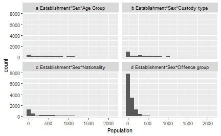
```

![](Week-5-Import-and-wrangling_files/figure-html/unnamed-chunk-18-1.png)
]

---
background-image: url(images/05/dplyr-logo.png)
background-size: 6%
background-position: 90% 5%

# Filtering rows

We can use the **filter()** function to select only the rows we're interested in, using *logical conditions* and *relational operators*.

```r
filter(prison_pop,
       View == "a Establishment*Sex*Age Group")
```

```
## # A tibble: 2,042 x 6
##    View                       Date    Establishment Sex    `Age / Custody / Nationality / Offence G~ Population
##    <chr>                      <chr>   <chr>         <chr>  <chr>                                          <dbl>
##  1 a Establishment*Sex*Age G~ 2015-06 Altcourse     Male   Adults (21+)                                     922
##  2 a Establishment*Sex*Age G~ 2015-06 Altcourse     Male   Juveniles and Young Adults (15-20)               169
##  3 a Establishment*Sex*Age G~ 2015-06 Ashfield      Male   Adults (21+)                                     389
##  4 a Establishment*Sex*Age G~ 2015-06 Askham Grange Female Adults (21+)                                      NA
##  5 a Establishment*Sex*Age G~ 2015-06 Askham Grange Female Juveniles and Young Adults (15-20)                NA
##  6 a Establishment*Sex*Age G~ 2015-06 Aylesbury     Male   Adults (21+)                                     113
##  7 a Establishment*Sex*Age G~ 2015-06 Aylesbury     Male   Juveniles and Young Adults (15-20)               268
##  8 a Establishment*Sex*Age G~ 2015-06 Bedford       Male   Adults (21+)                                     459
##  9 a Establishment*Sex*Age G~ 2015-06 Bedford       Male   Juveniles and Young Adults (15-20)                30
## 10 a Establishment*Sex*Age G~ 2015-06 Belmarsh      Male   Adults (21+)                                     794
## # ... with 2,032 more rows
```

---
# Relational operators

Relational operators compare two (or more) things and return a **logical** value (i.e. TRUE/FALSE)

|Operator|Meaning| Example|
|---|------------------| |
|>  | Greater than    |5 > 4|
|>= | Greater than or equal to| 4 >= 4|
|<  | Less than | Population < 400|
|<= | Less than or equal to | Population <= 400|
|== | Exactly equal to | Sex == "Male"| 
|!= | Not equal to | Establishment != "Ashfield"|
|%in%| Is contained in| Establishment %in% c("Bedford", "Oakwood")|

---
# Logical operators

Logical operators can be used to combine multiple relational operators or *negate* a relational operator.

|Operator| Meaning| Example|
|-|-|-|-|
|&| AND| Population < 1000 & Sex == "Male"|
|&#124;| OR| Population > 200 &vert; Population < 500|
|!| NOT| !(Establishment %in% c("Bedford", "Oakwood")) |

---
background-image: url(images/05/dplyr-logo.png)
background-size: 6%
background-position: 90% 5%

# Filtering rows

We can have multiple *conditions* for selection with **filter()**.

Suppose we only wanted to include rows where Population is over 300 but under 600.

```r
filter(prison_pop,
       View == "a Establishment*Sex*Age Group",
       Population > 300 & Population < 600)
```

```
## # A tibble: 487 x 6
##    View                       Date    Establishment Sex    `Age / Custody / Nationality / Offence G~ Population
##    <chr>                      <chr>   <chr>         <chr>  <chr>                                          <dbl>
##  1 a Establishment*Sex*Age G~ 2015-06 Ashfield      Male   Adults (21+)                                     389
##  2 a Establishment*Sex*Age G~ 2015-06 Bedford       Male   Adults (21+)                                     459
##  3 a Establishment*Sex*Age G~ 2015-06 Brinsford     Male   Juveniles and Young Adults (15-20)               349
##  4 a Establishment*Sex*Age G~ 2015-06 Bristol       Male   Adults (21+)                                     553
##  5 a Establishment*Sex*Age G~ 2015-06 Bronzefield   Female Adults (21+)                                     459
##  6 a Establishment*Sex*Age G~ 2015-06 Buckley Hall  Male   Adults (21+)                                     440
##  7 a Establishment*Sex*Age G~ 2015-06 Coldingley    Male   Adults (21+)                                     515
##  8 a Establishment*Sex*Age G~ 2015-06 Deerbolt      Male   Juveniles and Young Adults (15-20)               311
##  9 a Establishment*Sex*Age G~ 2015-06 Eastwood Park Female Adults (21+)                                     331
## 10 a Establishment*Sex*Age G~ 2015-06 Erlestoke     Male   Adults (21+)                                     514
## # ... with 477 more rows
```

---
class: inverse, middle, center
# Putting it all together

---
background-image: url(images/05/dplyr-logo.png)
background-size: 6%
background-position: 90% 5%

# Pipes

Often you want to conduct several steps, one after the other.

You could do this using objects to store each intermediate step.

```r
temp_pris <- filter(prison_pop,
                    View == "a Establishment*Sex*Age Group",
                    Date == "2015-06")
temp_pris <- group_by(temp_pris,
                      Sex,
                      `Age / Custody / Nationality / Offence Group`)
temp_pris <- summarise(temp_pris,
                       mean_pop = mean(Population, na.rm = TRUE), 
                       median_pop = median(Population, na.rm = TRUE),
                       total_pop = sum(Population, na.rm = TRUE),
                       max_pop = max(Population, na.rm = TRUE))
```

```
## `summarise()` regrouping output by 'Sex' (override with `.groups` argument)
```
---
background-image: url(images/05/dplyr-logo.png)
background-size: 6%
background-position: 90% 5%

# Pipes

A simpler way is to use *pipes* (**%>%**)

*pipes* can be read as meaning "AND THEN"

```r
prison_pop %>%
  filter(View == "a Establishment*Sex*Age Group",
         Date == "2015-06") %>%
  group_by(Sex, `Age / Custody / Nationality / Offence Group`) %>%
  summarise(mean_pop = mean(Population, na.rm = TRUE), 
            median_pop = median(Population, na.rm = TRUE),
            total_pop = sum(Population, na.rm = TRUE),
            max_pop = max(Population, na.rm = TRUE))
```

```
## `summarise()` regrouping output by 'Sex' (override with `.groups` argument)
```

```
## # A tibble: 4 x 6
## # Groups:   Sex [2]
##   Sex    `Age / Custody / Nationality / Offence Group` mean_pop median_pop total_pop max_pop
##   <chr>  <chr>                                            <dbl>      <dbl>     <dbl>   <dbl>
## 1 Female Adults (21+)                                     356          333      3560     480
## 2 Female Juveniles and Young Adults (15-20)                18.6         19       167      35
## 3 Male   Adults (21+)                                     717.         677     76730    1587
## 4 Male   Juveniles and Young Adults (15-20)               101.          54      5559     490
```

---
# Reading materials

## Revision

For revision of this week's concepts, see Chapter *Data transformation* in R for Data Science.

For practice, use the "Work with Data" RStudio cloud primer.

## Next week

Discovering Statistics using R (Field et al.)
  - Chapter 9, Comparing two means
  - Chapter 5, Exploring assumptions (additional)