class: center, middle, inverse, title-slide # Correlation and regression ### 1/12/2020 --- # Null Hypothesis Significance Testing (NHST) .large[ Think back to our previous questions: 1. Do men and women differ in terms of their fear of crime? 2. Are people who have been a victim of crime more fearful of crime? The basis of NHST is to phrase these questions as: If there is only one population, how likely is it that our two samples have values this different from each other? ] --- # Performing *t*-tests in R .pull-left[ The tilde (~) symbol in R usually means "modelled by" `FoC ~ victim_crime` means `FoC modelled by victim_crime`. `data = crime` tells R to look in the `crime` data frame for the data. `paired = FALSE` tells R that this is an *independent samples* test. ] .pull-right[ ```r t.test(FoC ~ victim_crime, data = crime, paired = FALSE) ``` ``` ## ## Welch Two Sample t-test ## ## data: FoC by victim_crime ## t = 0.45309, df = 197.48, p-value = 0.651 ## alternative hypothesis: true difference in means is not equal to 0 ## 95 percent confidence interval: ## -0.1873001 0.2990388 ## sample estimates: ## mean in group no mean in group yes ## 2.463636 2.407767 ``` ] --- class: inverse, middle, center # Correlation and statistical relationships --- # Correlation .large[ Correlation measures the strength and direction of an association between two continuous variables. ] .center[ 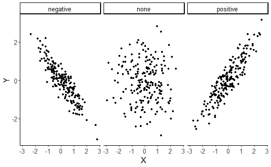<!-- --> ] --- # Correlation How related are the variables in the Fear of Crime dataset? ```r head(crime) ``` ``` ## # A tibble: 6 x 15 ## Participant sex age victim_crime H E X A C O SA TA OHQ FoC Foc2 ## <chr> <chr> <dbl> <chr> <dbl> <dbl> <dbl> <dbl> <dbl> <dbl> <dbl> <dbl> <dbl> <dbl> <dbl> ## 1 R_01TjXgC191rVSst male 55 yes 3.7 3 3.4 3.9 3.2 3.6 1.15 1.55 3.41 2.6 3 ## 2 R_0dN5YeULcyms2qN female 20 no 2.5 3.1 2.5 2.4 2.2 3.1 2.05 2.95 2.38 2 3 ## 3 R_0DPiPYWhncWS1TX male 57 yes 2.6 3.1 3.3 3.1 4.3 2.8 2 2.6 3 1.2 2 ## 4 R_0f7bSsH6Up0yelz male 19 no 3.5 1.8 3.3 3.4 2.1 2.7 1.55 2.1 3.48 3.2 5 ## 5 R_0rov2RoSkPEOvlv female 20 no 3.3 3.4 3.9 3.2 2.8 3.9 1.3 1.8 3.59 2.8 3 ## 6 R_0wioqGERxElVTh3 female 20 no 2.6 2.6 3 2.6 2.9 3.4 2.55 1.5 3.76 2 4 ``` --- # Correlation .pull-left[ Let's look at the relationship between Emotionality (*E*) and Fear of Crime (*FoC*). ```r ggplot(crime, aes(x = E, y = FoC)) + geom_jitter() + theme_classic(base_size = 20) + labs(x = "Emotionality", y = "Fear of Crime") ``` ] .pull-right[ 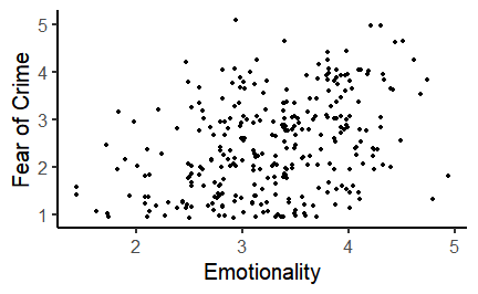 ] --- # Correlation and covariance .pull-left[ .large[ How do we quantify the relationship between these variables? We need to look at how much they *vary together*. The plot shows the Emotionality values of the first ten participants. The line across the middle is the mean of those values - **2.9**. ] ] .pull-right[ 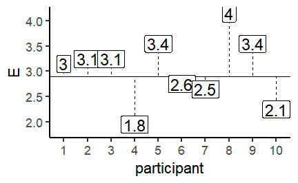<!-- --> ] --- # The mean and the variance .pull-left[ As you can see, the values don't lie directly on the mean, but are spread around it. To quantify how much the values vary from the mean, we can calculate the *variance*. Here's the scary looking formula for the variance: $$ \sigma^2 = \frac{\sum(x - \bar{x})^2}{N - 1} $$ And here's the not-so-scary R function: ```r var(x) ``` ] .pull-right[ <!-- --> ] --- # Correlation and covariance .pull-left[ .large[ Now let's look at the same plot for Fear of Crime (FoC). Again, these points and labels are individual ratings of Fear of Crime. The line across the middle shows the mean, which is **2.22**. ] ] .pull-right[ 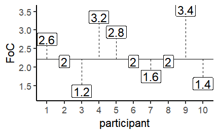<!-- --> ] --- # Correlation and covariance .pull-left[ Now let's look at these previous two plots as differences from their respective means. What we want to now is to what extent the values *vary together*. I.e. as one goes up, does the other? This is *covariance*. Here's the scary formula: $$ cov(x, y) = \frac{\sum((x - \bar{x})(y - \bar{y}))}{N - 1} $$ Here's the not-so-scary R function: ```r cov(x, y) ``` ] .pull-right[ <!-- --> ] --- # Correlation and covariance .pull-left[ Covariance gives us a measure of how much two variables vary together. But the numbers it gives us can be hard to interpret when the variables are on very different scales. So we rescale the covariance using the standard deviations of each variable. $$ corr(x, y) = r = \frac{cov(x, y)}{\sigma^x\sigma^y} $$ This gives us the *correlation coefficient*, or *r*. ```r cor(crime$E, crime$FoC) ``` ``` ## [1] 0.369891 ``` ] .pull-right[ ``` ## `geom_smooth()` using formula 'y ~ x' ``` <!-- --> ] --- # Pearson's product-moment correlation The **cor.test()** function can be used to test the *significance* of a correlation. ```r cor.test(crime$E, crime$FoC, method = "pearson") ``` ``` ## ## Pearson's product-moment correlation ## ## data: crime$E and crime$FoC *## t = 6.8843, df = 299, p-value = 3.421e-11 ## alternative hypothesis: true correlation is not equal to 0 ## 95 percent confidence interval: *## 0.2680476 0.4635586 ## sample estimates: ## cor *## 0.369891 ``` --- # Curved or non-linear relationships If your data look like this: .pull-left[ <!-- --> ] .pull-right[ <!-- --> ] ...forget about correlation. --- # Curved or non-linear relationships .pull-left[ ...but if your data look like this: 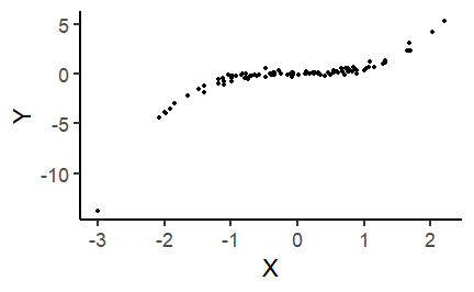<!-- --> ...there is some hope! ] .pull-right[ Spearman's rank correlation is used to measure *monotonicity*, and is the non-parametric equivalent to Pearson's correlation. If the data is not already ranks then it is converted to ranks; then the ranks are correlated across variables. ```r cor.test(X, Y, method = "spearman") ``` ``` ## ## Spearman's rank correlation rho ## ## data: X and Y *## S = 17494, p-value < 2.2e-16 ## alternative hypothesis: true rho is not equal to 0 ## sample estimates: ## rho *## 0.8950255 ``` ] --- background-image: url(images/07/chart.png) background-size: 80% background-position: 50% 70% # Correlation is not causation [https://www.spuriouscorrelations.com](https://www.spuriouscorrelations.com) --- # Reporting a correlation .large[ Reporting a correlation is pretty straightforward. Only the correlation coefficient and p-value are typically required. e.g. "There was a significant positive correlation between emotionality and fear of crime, *r* = .37, *p* < .001." However, it's best to also specify which type of correlation you used (e.g. Pearson's or Spearman's); and a scatterplot showing the relationship should almost always be shown. Typically, the degrees of freedom or number of observations should also be given, e.g. *r*(299) = .37, *p* < .001, or r = .37, *p* < .001, *N* = 301. Note that *r* is considered a measure of *effect size*. An *r* of .1 is considered a small effect, while an *r* of .8 is considered a large effect. ] --- class: inverse, middle, center # Linear regression --- # Correlation, regression and prediction .pull-left[ Correlation quantifies the *strength* and *direction* of an association between two continuous variables. But what if we want to *predict* the values of one variable from those of another? For example, as Emotionality increases, *how much* does Fear of Crime change? ```r ggplot(crime, aes(x = E, y = FoC)) + geom_jitter() + stat_smooth(method = "lm", se = FALSE) + theme_classic(base_size = 22) + labs(x = "Emotionality", y = "Fear of crime") ``` ``` ## `geom_smooth()` using formula 'y ~ x' ``` ] .pull-right[ 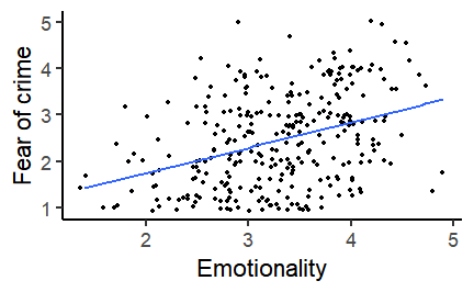 ] --- # Linear regression .pull-left[  ] .pull-right[ .large[ The line added to this scatterplot is the *line of best fit*. It's the straight line that gets closest to going through all of the points on the plot. But how do we work out where the line should be? ] ] --- # The line of best fit The line represents the predicted value of **y** at each value of **x**. The prediction is made using the following formula: `\(y = a + bX\)` *a* is the *intercept* - the point where the line would cross the y-axis when the value of the x-axis is 0. *b* is the *slope* - the steepness and direction of the line. The *line of best fit* can be found by adjusting the *intercept* and *slope* to minimise the *sum of squared residuals*. [Line of best fit demo](https://shinyapps.org/showapp.php?app=https://tellmi.psy.lmu.de/felix/lmfit&by=Felix%20Sch%C3%B6nbrodt&title=Find-a-fit!&shorttitle=Find-a-fit!) --- # Fear of crime predicted by emotionality .pull-left[ Let's try using the **lm()** function to predict Fear of Crime (*FoC*) from Emotionality (*E*). ```r foc_by_E <- lm(FoC ~ E, data = crime) foc_by_E ``` ``` ## ## Call: ## lm(formula = FoC ~ E, data = crime) ## *## Coefficients: *## (Intercept) E *## 0.6492 0.5475 ``` These are the *intercept* and *slope* of the regression line on the right. ] .pull-right[ ``` ## `geom_smooth()` using formula 'y ~ x' ``` 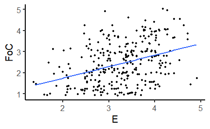<!-- --> ] --- # Is this a good model of Fear of crime? ```r summary(foc_by_E) ``` ``` ## ## Call: ## lm(formula = FoC ~ E, data = crime) ## ## Residuals: ## Min 1Q Median 3Q Max ## -1.87698 -0.72952 -0.03902 0.70844 2.76319 ## ## Coefficients: *## Estimate Std. Error t value Pr(>|t|) *## (Intercept) 0.64918 0.26621 2.439 0.0153 * *## E 0.54746 0.07952 6.884 3.42e-11 *** ## --- ## Signif. codes: 0 '***' 0.001 '**' 0.01 '*' 0.05 '.' 0.1 ' ' 1 ## *## Residual standard error: 0.9278 on 299 degrees of freedom *## Multiple R-squared: 0.1368, Adjusted R-squared: 0.1339 *## F-statistic: 47.39 on 1 and 299 DF, p-value: 3.421e-11 ``` --- # Fear of crime predicted by emotionality Let's focus on the coefficients. ```r summary(foc_by_E)$coefficients ``` ``` ## Estimate Std. Error t value Pr(>|t|) ## (Intercept) 0.6491774 0.26621482 2.438547 1.532835e-02 ## E 0.5474598 0.07952319 6.884279 3.421376e-11 ``` Estimate is the *coefficient* of each predictor; Std. Error is an estimate of the accuracy of that coefficient. The significance of each predictor is tested using a t-test; *t value* is the t statistic, and the *Pr(>|t|)* column is the p-value. Thus, *Emotionality* is a significant predictor of *Fear of Crime*. Since its coefficient is positive, Fear of Crime increases as Emotionality increases. --- # Fear of crime predicted by emotionality .pull-left[ Again, the regression line is described by the formula `\(y = a + bX\)`. So we can fill that out with our model coefficients as follows: Fear of crime = 0.65 + 0.55 * `\(X\)` `\(X\)` is the value of the *predictor*. The *intercept* is now the value of `\(y\)` when the value of the predictor is *zero*. The coefficient for the predictor is the amount that `\(y\)` increases for each 1 unit increase in the predictor. ] .pull-right[ ``` ## `geom_smooth()` using formula 'y ~ x' ``` 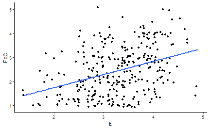<!-- --> ] --- class: inverse, center, middle # Assessing model significance --- # Is this a good model? ```r summary(foc_by_E) ``` ``` ## ## Call: ## lm(formula = FoC ~ E, data = crime) ## ## Residuals: ## Min 1Q Median 3Q Max ## -1.87698 -0.72952 -0.03902 0.70844 2.76319 ## ## Coefficients: ## Estimate Std. Error t value Pr(>|t|) ## (Intercept) 0.64918 0.26621 2.439 0.0153 * ## E 0.54746 0.07952 6.884 3.42e-11 *** ## --- ## Signif. codes: 0 '***' 0.001 '**' 0.01 '*' 0.05 '.' 0.1 ' ' 1 ## *## Residual standard error: 0.9278 on 299 degrees of freedom *## Multiple R-squared: 0.1368, Adjusted R-squared: 0.1339 *## F-statistic: 47.39 on 1 and 299 DF, p-value: 3.421e-11 ``` --- # The mean as a model .pull-left[ First, let's create a linear model that simply finds the *mean* using the **lm()** function. ```r intercept_only <- lm(FoC ~ 1, data = crime) intercept_only ``` ``` ## ## Call: ## lm(formula = FoC ~ 1, data = crime) ## *## Coefficients: *## (Intercept) *## 2.445 ``` Here the Intercept is equal to the *mean* of FoC. ```r mean(crime$FoC) ``` ``` ## [1] 2.444518 ``` ] .pull-right[ In the formula `\(y = a + bX\)`, *a* is the *Intercept*. So our prediction for the value of *y* is `\(y = 2.44\)`. <!-- --> ] --- #The mean as a model ```r summary(intercept_only) ``` ``` ## ## Call: ## lm(formula = FoC ~ 1, data = crime) ## ## Residuals: ## Min 1Q Median 3Q Max ## -1.44452 -0.84452 -0.04452 0.55548 2.55548 ## ## Coefficients: *## Estimate Std. Error t value Pr(>|t|) *## (Intercept) 2.44452 0.05746 42.54 <2e-16 *** ## --- ## Signif. codes: 0 '***' 0.001 '**' 0.01 '*' 0.05 '.' 0.1 ' ' 1 ## *## Residual standard error: 0.9969 on 300 degrees of freedom ``` --- #Model comparison We can compare models using the **anova()** function. ```r anova(intercept_only, foc_by_E) ``` ``` ## Analysis of Variance Table ## ## Model 1: FoC ~ 1 ## Model 2: FoC ~ E ## Res.Df RSS Df Sum of Sq F Pr(>F) ## 1 300 298.16 ## 2 299 257.37 1 40.795 47.393 3.421e-11 *** ## --- ## Signif. codes: 0 '***' 0.001 '**' 0.01 '*' 0.05 '.' 0.1 ' ' 1 ``` ```r summary(foc_by_E)$fstatistic ``` ``` ## value numdf dendf ## 47.3933 1.0000 299.0000 ``` --- # At least it's better than the mean! ```r summary(foc_by_E) ``` ``` ## ## Call: ## lm(formula = FoC ~ E, data = crime) ## ## Residuals: ## Min 1Q Median 3Q Max ## -1.87698 -0.72952 -0.03902 0.70844 2.76319 ## ## Coefficients: ## Estimate Std. Error t value Pr(>|t|) ## (Intercept) 0.64918 0.26621 2.439 0.0153 * ## E 0.54746 0.07952 6.884 3.42e-11 *** ## --- ## Signif. codes: 0 '***' 0.001 '**' 0.01 '*' 0.05 '.' 0.1 ' ' 1 ## ## Residual standard error: 0.9278 on 299 degrees of freedom ## Multiple R-squared: 0.1368, Adjusted R-squared: 0.1339 *## F-statistic: 47.39 on 1 and 299 DF, p-value: 3.421e-11 ``` --- class: inverse, center, middle # Assessing model fit --- # How much does Y does X explain? ```r summary(foc_by_E) ``` ``` ## ## Call: ## lm(formula = FoC ~ E, data = crime) ## ## Residuals: ## Min 1Q Median 3Q Max ## -1.87698 -0.72952 -0.03902 0.70844 2.76319 ## ## Coefficients: ## Estimate Std. Error t value Pr(>|t|) ## (Intercept) 0.64918 0.26621 2.439 0.0153 * ## E 0.54746 0.07952 6.884 3.42e-11 *** ## --- ## Signif. codes: 0 '***' 0.001 '**' 0.01 '*' 0.05 '.' 0.1 ' ' 1 ## ## Residual standard error: 0.9278 on 299 degrees of freedom *## Multiple R-squared: 0.1368, Adjusted R-squared: 0.1339 ## F-statistic: 47.39 on 1 and 299 DF, p-value: 3.421e-11 ``` --- # Model fit .pull-left[ .large[ R-squared ( `\(R^2\)` ) is a measure of model fit. Specifically, it's the proportion of *explained* variance in the data. We previously looked at the *variance* around the *mean*. After linear regression, we look at how much reality differs from the model predictions - the *residual error*. ] ] .pull-right[ <!-- --> ] --- # Model fit .pull-left[ .large[ To work out how well our model fits, we first need to know how much *total variation* there is in the data. For that, we sum the squared differences of the values of the dependent variable `\(y\)` from the mean of the dependent variable `\(\bar{y}\)` - the *total sum of squares*, `\(SS_t\)`: `\(SS_t = \sum(y - \bar{y})^2\)` ] ] .pull-right[ <!-- --> ] --- # Squared differences .pull-left[ .large[ Why square the differences? 1. Negative values become positive. 2. Values that are further away from the mean often get even further away. This prevents "errors" from cancelling out, and effectively penalises values that are far away from the mean. ] ] .pull-right[  ] --- # Model fit .pull-left[ .large[ We then calculate the sum of the squared differences of the values of the dependent variable ( `\(y\)` ) from the model predictions - the sum of the squared residuals, `\(SS_r\)`: `\(SS_r = \sum(y - \hat{y})^2\)` ] ] .pull-right[ <!-- --> ] --- # Model fit .large[ Finally, we calculate *model sum of squares* - `\(SS_m\)` - as the difference between the *total sum of squares* and the *residual sum of squares*. This tells us, roughly, how much better our model is than just using the *mean*: `\(SS_m = SS_t - SS_r\)` R-squared ( `\(R^2\)` ) can then be calculated by dividing the model sum of squares by the total sum of squares: `\(R^2 = \frac{SS_m}{SS_t}\)` This yields the *percentage of variance explained by the model*. This is a long-winded way of saying: Higher `\(R^2\)` means more explained variance, and thus, a better fitting model. ] --- # Model fit .large[ Thankfully, R does all these calculations for us! ```r summary(foc_by_E)$r.squared ``` ``` ## [1] 0.1368193 ``` Our simple regression model of the effect of Emotionality on Fear of Crime explained ~ 14% of the variance. What's left? 1. Other variables? 2. Measurement error? ] --- class: center, middle, inverse # Reporting simple regression --- # Example of reporting a simple regression model .large[ "Simple linear regression was used to investigate the relationship between emotionality and fear of crime. A significant regression equation was found that explained 14% of the variance, `\(R^2\)` = .14, *F*(1, 299) = 47.39, *p* < .001. Fear of crime also increased significantly with increases in Emotionality, `\(B\)` = 0.55, t(6.884), p < .001." ] --- # Nicely formatted tables using stargazer... ```r library(stargazer) stargazer(foc_by_E, single.row = TRUE, type = "html") ``` <table style="text-align:center"><tr><td colspan="2" style="border-bottom: 1px solid black"></td></tr><tr><td style="text-align:left"></td><td><em>Dependent variable:</em></td></tr> <tr><td></td><td colspan="1" style="border-bottom: 1px solid black"></td></tr> <tr><td style="text-align:left"></td><td>FoC</td></tr> <tr><td colspan="2" style="border-bottom: 1px solid black"></td></tr><tr><td style="text-align:left">E</td><td>0.547<sup>***</sup> (0.080)</td></tr> <tr><td style="text-align:left">Constant</td><td>0.649<sup>**</sup> (0.266)</td></tr> <tr><td colspan="2" style="border-bottom: 1px solid black"></td></tr><tr><td style="text-align:left">Observations</td><td>301</td></tr> <tr><td style="text-align:left">R<sup>2</sup></td><td>0.137</td></tr> <tr><td style="text-align:left">Adjusted R<sup>2</sup></td><td>0.134</td></tr> <tr><td style="text-align:left">Residual Std. Error</td><td>0.928 (df = 299)</td></tr> <tr><td style="text-align:left">F Statistic</td><td>47.393<sup>***</sup> (df = 1; 299)</td></tr> <tr><td colspan="2" style="border-bottom: 1px solid black"></td></tr><tr><td style="text-align:left"><em>Note:</em></td><td style="text-align:right"><sup>*</sup>p<0.1; <sup>**</sup>p<0.05; <sup>***</sup>p<0.01</td></tr> </table> --- #... or using sjPlot ```r library(sjPlot) tab_model(foc_by_E, show.std = TRUE, title = "Table 1: Linear regression model", pred.labels = c("Intercept", "Emotionality"), dv.labels = "Fear of Crime", show.fstat = TRUE) ``` <table style="border-collapse:collapse; border:none;"> <caption style="font-weight: bold; text-align:left;">Table 1: Linear regression model</caption> <tr> <th style="border-top: double; text-align:center; font-style:normal; font-weight:bold; padding:0.2cm; text-align:left; "> </th> <th colspan="5" style="border-top: double; text-align:center; font-style:normal; font-weight:bold; padding:0.2cm; ">Fear of Crime</th> </tr> <tr> <td style=" text-align:center; border-bottom:1px solid; font-style:italic; font-weight:normal; text-align:left; ">Predictors</td> <td style=" text-align:center; border-bottom:1px solid; font-style:italic; font-weight:normal; ">Estimates</td> <td style=" text-align:center; border-bottom:1px solid; font-style:italic; font-weight:normal; ">std. Beta</td> <td style=" text-align:center; border-bottom:1px solid; font-style:italic; font-weight:normal; ">CI</td> <td style=" text-align:center; border-bottom:1px solid; font-style:italic; font-weight:normal; ">standardized CI</td> <td style=" text-align:center; border-bottom:1px solid; font-style:italic; font-weight:normal; ">p</td> </tr> <tr> <td style=" padding:0.2cm; text-align:left; vertical-align:top; text-align:left; ">Intercept</td> <td style=" padding:0.2cm; text-align:left; vertical-align:top; text-align:center; ">0.65</td> <td style=" padding:0.2cm; text-align:left; vertical-align:top; text-align:center; ">0.00</td> <td style=" padding:0.2cm; text-align:left; vertical-align:top; text-align:center; ">0.13 – 1.17</td> <td style=" padding:0.2cm; text-align:left; vertical-align:top; text-align:center; ">-0.11 – 0.11</td> <td style=" padding:0.2cm; text-align:left; vertical-align:top; text-align:center; "><strong>0.015</strong></td> </tr> <tr> <td style=" padding:0.2cm; text-align:left; vertical-align:top; text-align:left; ">Emotionality</td> <td style=" padding:0.2cm; text-align:left; vertical-align:top; text-align:center; ">0.55</td> <td style=" padding:0.2cm; text-align:left; vertical-align:top; text-align:center; ">0.37</td> <td style=" padding:0.2cm; text-align:left; vertical-align:top; text-align:center; ">0.39 – 0.70</td> <td style=" padding:0.2cm; text-align:left; vertical-align:top; text-align:center; ">0.26 – 0.48</td> <td style=" padding:0.2cm; text-align:left; vertical-align:top; text-align:center; "><strong><0.001</td> </tr> <tr> <td style=" padding:0.2cm; text-align:left; vertical-align:top; text-align:left; padding-top:0.1cm; padding-bottom:0.1cm; border-top:1px solid;">Observations</td> <td style=" padding:0.2cm; text-align:left; vertical-align:top; padding-top:0.1cm; padding-bottom:0.1cm; text-align:left; border-top:1px solid;" colspan="5">301</td> </tr> <tr> <td style=" padding:0.2cm; text-align:left; vertical-align:top; text-align:left; padding-top:0.1cm; padding-bottom:0.1cm;">R<sup>2</sup> / R<sup>2</sup> adjusted</td> <td style=" padding:0.2cm; text-align:left; vertical-align:top; padding-top:0.1cm; padding-bottom:0.1cm; text-align:left;" colspan="5">0.137 / 0.134</td> </tr> </table> --- # Next week Next week we'll continue with **regression**, looking at multiple predictors. We'll also begin with **one-way ANOVA** for comparison of multiple means. ## Reading Chapter 10 - Comparing Several Means - ANOVA (GLM 1) --- # Additional support Maths & Stats Help (AKA MASH) are a service offered by the University, based over in the library. They offer support to both undergraduate and postgraduate students. You'll find their website at [https://guides.library.lincoln.ac.uk/mash](https://guides.library.lincoln.ac.uk/mash) Note that while their website is mostly about other software, they do support R! Or join the MS Teams group, use the discussion board, or drop me an email!