class: center, middle, inverse, title-slide # Multiple predictors and multiple means ### 7/12/2021 --- # Different correlations 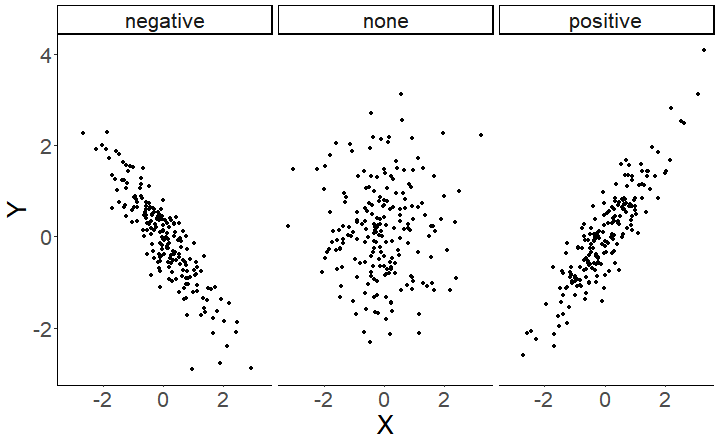<!-- --> --- # Correlation summary .large[ Correlation coefficients are bound in a range from -1 to 1. Negative coefficients mean that as one variable increases, the other decreases. Positive coefficients mean that as one variable increases, the other also increases. ] 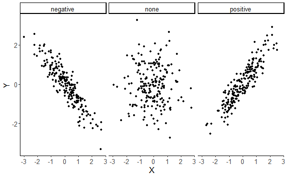<!-- --> --- #Correlation, regression and prediction .pull-left[ Correlation quantifies the *strength* and *direction* of an association between two continuous variables. But what if we want to *predict* the values of one variable from those of another? For example, as Emotionality increases, *how much* does Fear of Crime change? ```r ggplot(crime, aes(x = E, y = FoC)) + geom_point() + stat_smooth(method = "lm", se = FALSE) + theme_classic() + labs(x = "Emotionality", y = "Fear of crime") ``` ``` ## `geom_smooth()` using formula 'y ~ x' ``` ] .pull-right[ 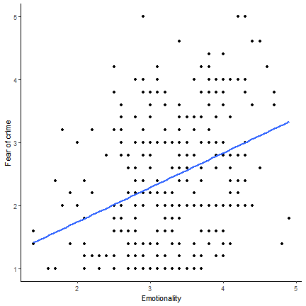 ] --- # Simple linear regression .pull-left[  ] .pull-right[ The line added to this scatterplot is the *line of best fit*. A line like this can be described by two parameters - the *intercept* and the *slope*. The *intercept* is where the line crosses the *y-axis*. The *slope* is the *steepness* of the line. Given these parameters, we can predict the value of **y** - the dependent variable - at each value of **x** - the independent, predictor variable - using the following formula: `\(y = a + bX\)` ] --- class: inverse, middle, center # Multiple linear regression --- # Predicting children's reading ability .pull-left[ ```r child_data <- read_csv("data/child_data.csv") head(child_data) ``` ``` ## # A tibble: 6 x 5 ## participant IQ age mem_span read_ab ## <dbl> <dbl> <dbl> <dbl> <dbl> ## 1 1 93 7.3 4.2 7.27 ## 2 2 93 5.4 3.8 5.29 ## 3 3 97 7.3 4.7 7.83 ## 4 4 89 4 3.4 6.22 ## 5 5 91 5.8 3.8 6.62 ## 6 6 95 7.8 4.4 7.02 ``` ] .pull-right[ .large[ This data is from a study investigating whether children's reading ability can be predicted from their working memory capacity. ] ] --- # Predicting children's reading ability .pull-left[ As a starting point, we look at a plot of the relationship between memory span and reading ability, which suggests a positive relationship between the two variables. ```r ggplot(child_data, aes(x = mem_span, y = read_ab)) + geom_point() + stat_smooth(method = "lm") ``` ``` ## `geom_smooth()` using formula 'y ~ x' ``` ] .pull-right[ 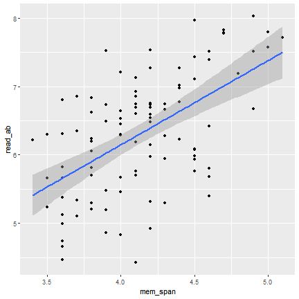 ] --- # Simple linear regression ```r simple_model <- lm(read_ab ~ mem_span, data = child_data) summary(simple_model) ``` ``` ## ## Call: ## lm(formula = read_ab ~ mem_span, data = child_data) ## ## Residuals: ## Min 1Q Median 3Q Max ## -1.8492 -0.5742 0.1536 0.5252 1.4998 ## ## Coefficients: ## Estimate Std. Error t value Pr(>|t|) ## (Intercept) 1.2356 0.7580 1.630 0.106 *## mem_span 1.2283 0.1826 6.726 1.17e-09 *** ## --- ## Signif. codes: 0 '***' 0.001 '**' 0.01 '*' 0.05 '.' 0.1 ' ' 1 ## ## Residual standard error: 0.7198 on 98 degrees of freedom ## Multiple R-squared: 0.3158, Adjusted R-squared: 0.3089 *## F-statistic: 45.24 on 1 and 98 DF, p-value: 1.172e-09 ``` --- # Simple vs multiple regression .pull-left[ 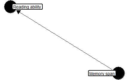<!-- --> ] -- .pull-right[ 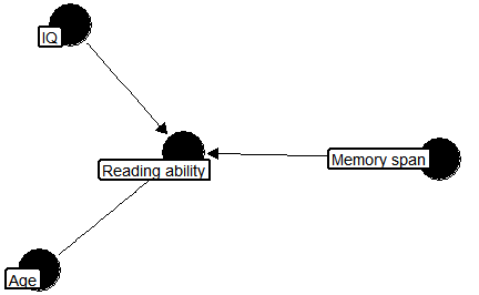<!-- --> ] --- # Simple vs multiple regression .pull-left[ 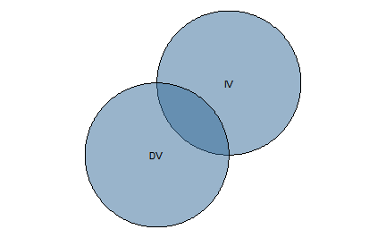<!-- --> ] -- .pull-right[ 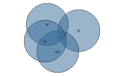<!-- --> ] --- # Expanding our equation .pull-left[ Multiple linear regression deals with multiple predictors. The *bX* in our regression equation - `\(y = a + bX + \varepsilon\)` - can be expanded. For example, with two predictors, our equation would be: `\(y = a_0 + b_1 \times X_1 + b_2 \times X_2 + \varepsilon\)` ```r a <- 2 # Our intercept term b1 <- 0.65 # Our first regression coefficient X1 <- rnorm(1000, 6, 1) # Our first predictor b2 <- -0.8 # Our second regression coefficient X2 <- rnorm(1000, 3, 1) # Our second predictor err <- rnorm(1000, 0, 1) # Our error term y <- a + b1 * X1 + b2 * X2 + err # Our response variable ``` ] .pull-right[ ``` ## `geom_smooth()` using formula 'y ~ x' ``` 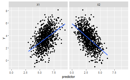<!-- --> ] --- # Multiple linear regression ```r full_model <- lm(read_ab ~ mem_span + age + IQ, data = child_data) summary(full_model) ``` ``` ## ## Call: ## lm(formula = read_ab ~ mem_span + age + IQ, data = child_data) ## ## Residuals: ## Min 1Q Median 3Q Max ## -1.31874 -0.50709 0.03617 0.49949 1.25350 ## ## Coefficients: ## Estimate Std. Error t value Pr(>|t|) ## (Intercept) 2.96025 1.45449 2.035 0.04458 * *## mem_span 0.64429 0.29462 2.187 0.03118 * *## age 0.30835 0.09833 3.136 0.00228 ** *## IQ -0.01217 0.01704 -0.714 0.47666 ## --- ## Signif. codes: 0 '***' 0.001 '**' 0.01 '*' 0.05 '.' 0.1 ' ' 1 ## ## Residual standard error: 0.6703 on 96 degrees of freedom ## Multiple R-squared: 0.4189, Adjusted R-squared: 0.4007 ## F-statistic: 23.07 on 3 and 96 DF, p-value: 2.503e-11 ``` --- # Is the more complex model better? We can explicitly compare models using the `anova()` function. ```r anova(simple_model, full_model) ``` ``` ## Analysis of Variance Table ## ## Model 1: read_ab ~ mem_span ## Model 2: read_ab ~ mem_span + age + IQ ## Res.Df RSS Df Sum of Sq F Pr(>F) ## 1 98 50.780 *## 2 96 43.133 2 7.6471 8.5101 0.0003959 *** ## --- ## Signif. codes: 0 '***' 0.001 '**' 0.01 '*' 0.05 '.' 0.1 ' ' 1 ``` --- # Comparing regression models An alternative way to compare models is using the Akaike Information Criterion. ```r AIC(simple_model) ``` ``` ## [1] 222.0207 ``` ```r AIC(full_model) ``` ``` ## [1] 209.6989 ``` AIC **penalizes** model complexity. A complex model that explains as much variance as a simple model is considered *worse*. Lower is better! --- # Comparing predictors .large[The relative size of a predictor's effect can't *(always)* be judged from their coefficients, since the variables can be on different *scales*. ```r full_model$coefficients ``` ``` ## (Intercept) mem_span age IQ ## 2.96025254 0.64428763 0.30834521 -0.01217206 ``` ``` ## # A tibble: 4 x 4 ## variable min max sd ## <chr> <dbl> <dbl> <dbl> ## 1 age 4 8 1.14 ## 2 IQ 89 108 4.83 ## 3 mem_span 3.4 5.1 0.396 ## 4 read_ab 4.42 8.03 0.866 ``` ] --- # Standardizing variables We can standardize our variables to put them on the same scale. The `scale()` function *mean-centres* and *scales* variables: it subtracts the mean and divides by the standard deviation. ``` ## Warning: attributes are not identical across measure variables; ## they will be dropped ``` 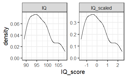<!-- --> --- ```r summary(lm(read_ab ~ mem_span + age + IQ, data = as.data.frame(scale(child_data)))) ``` ``` ## ## Call: ## lm(formula = read_ab ~ mem_span + age + IQ, data = as.data.frame(scale(child_data))) ## ## Residuals: ## Min 1Q Median 3Q Max ## -1.52302 -0.58564 0.04177 0.57687 1.44768 ## ## Coefficients: ## Estimate Std. Error t value Pr(>|t|) ## (Intercept) -2.703e-16 7.741e-02 0.000 1.00000 ## mem_span 2.948e-01 1.348e-01 2.187 0.03118 * ## age 4.043e-01 1.289e-01 3.136 0.00228 ** ## IQ -6.795e-02 9.510e-02 -0.714 0.47666 ## --- ## Signif. codes: 0 '***' 0.001 '**' 0.01 '*' 0.05 '.' 0.1 ' ' 1 ## ## Residual standard error: 0.7741 on 96 degrees of freedom ## Multiple R-squared: 0.4189, Adjusted R-squared: 0.4007 ## F-statistic: 23.07 on 3 and 96 DF, p-value: 2.503e-11 ``` --- # Standardized coefficients These coefficients now represent the change in the dependent variable from a **1 standard deviation** change from the **independent variable's mean**. sjPlot's `tab_model()` function can also do this for us: ```r tab_model(full_model, show.std = TRUE) ``` <table style="border-collapse:collapse; border:none;"> <tr> <th style="border-top: double; text-align:center; font-style:normal; font-weight:bold; padding:0.2cm; text-align:left; "> </th> <th colspan="5" style="border-top: double; text-align:center; font-style:normal; font-weight:bold; padding:0.2cm; ">read_ab</th> </tr> <tr> <td style=" text-align:center; border-bottom:1px solid; font-style:italic; font-weight:normal; text-align:left; ">Predictors</td> <td style=" text-align:center; border-bottom:1px solid; font-style:italic; font-weight:normal; ">Estimates</td> <td style=" text-align:center; border-bottom:1px solid; font-style:italic; font-weight:normal; ">std. Beta</td> <td style=" text-align:center; border-bottom:1px solid; font-style:italic; font-weight:normal; ">CI</td> <td style=" text-align:center; border-bottom:1px solid; font-style:italic; font-weight:normal; ">standardized CI</td> <td style=" text-align:center; border-bottom:1px solid; font-style:italic; font-weight:normal; ">p</td> </tr> <tr> <td style=" padding:0.2cm; text-align:left; vertical-align:top; text-align:left; ">(Intercept)</td> <td style=" padding:0.2cm; text-align:left; vertical-align:top; text-align:center; ">2.96</td> <td style=" padding:0.2cm; text-align:left; vertical-align:top; text-align:center; ">-0.00</td> <td style=" padding:0.2cm; text-align:left; vertical-align:top; text-align:center; ">0.07 – 5.85</td> <td style=" padding:0.2cm; text-align:left; vertical-align:top; text-align:center; ">-0.15 – 0.15</td> <td style=" padding:0.2cm; text-align:left; vertical-align:top; text-align:center; "><strong>0.045</strong></td> </tr> <tr> <td style=" padding:0.2cm; text-align:left; vertical-align:top; text-align:left; ">mem span</td> <td style=" padding:0.2cm; text-align:left; vertical-align:top; text-align:center; ">0.64</td> <td style=" padding:0.2cm; text-align:left; vertical-align:top; text-align:center; ">0.29</td> <td style=" padding:0.2cm; text-align:left; vertical-align:top; text-align:center; ">0.06 – 1.23</td> <td style=" padding:0.2cm; text-align:left; vertical-align:top; text-align:center; ">0.03 – 0.56</td> <td style=" padding:0.2cm; text-align:left; vertical-align:top; text-align:center; "><strong>0.031</strong></td> </tr> <tr> <td style=" padding:0.2cm; text-align:left; vertical-align:top; text-align:left; ">age</td> <td style=" padding:0.2cm; text-align:left; vertical-align:top; text-align:center; ">0.31</td> <td style=" padding:0.2cm; text-align:left; vertical-align:top; text-align:center; ">0.40</td> <td style=" padding:0.2cm; text-align:left; vertical-align:top; text-align:center; ">0.11 – 0.50</td> <td style=" padding:0.2cm; text-align:left; vertical-align:top; text-align:center; ">0.15 – 0.66</td> <td style=" padding:0.2cm; text-align:left; vertical-align:top; text-align:center; "><strong>0.002</strong></td> </tr> <tr> <td style=" padding:0.2cm; text-align:left; vertical-align:top; text-align:left; ">IQ</td> <td style=" padding:0.2cm; text-align:left; vertical-align:top; text-align:center; ">-0.01</td> <td style=" padding:0.2cm; text-align:left; vertical-align:top; text-align:center; ">-0.07</td> <td style=" padding:0.2cm; text-align:left; vertical-align:top; text-align:center; ">-0.05 – 0.02</td> <td style=" padding:0.2cm; text-align:left; vertical-align:top; text-align:center; ">-0.26 – 0.12</td> <td style=" padding:0.2cm; text-align:left; vertical-align:top; text-align:center; ">0.477</td> </tr> <tr> <td style=" padding:0.2cm; text-align:left; vertical-align:top; text-align:left; padding-top:0.1cm; padding-bottom:0.1cm; border-top:1px solid;">Observations</td> <td style=" padding:0.2cm; text-align:left; vertical-align:top; padding-top:0.1cm; padding-bottom:0.1cm; text-align:left; border-top:1px solid;" colspan="5">100</td> </tr> <tr> <td style=" padding:0.2cm; text-align:left; vertical-align:top; text-align:left; padding-top:0.1cm; padding-bottom:0.1cm;">R<sup>2</sup> / R<sup>2</sup> adjusted</td> <td style=" padding:0.2cm; text-align:left; vertical-align:top; padding-top:0.1cm; padding-bottom:0.1cm; text-align:left;" colspan="5">0.419 / 0.401</td> </tr> </table> --- class: inverse, middle, center # How to decide on your model --- # Which predictors should you include? If we look back at the Fear of Crime dataset, there are many potential predictors you could include. ```r head(crime) ``` ``` ## # A tibble: 6 x 15 ## Participant sex age victim_crime H E X A C O SA TA OHQ FoC ## <chr> <chr> <dbl> <chr> <dbl> <dbl> <dbl> <dbl> <dbl> <dbl> <dbl> <dbl> <dbl> <dbl> ## 1 R_01TjXgC191r~ male 55 yes 3.7 3 3.4 3.9 3.2 3.6 1.15 1.55 3.41 2.6 ## 2 R_0dN5YeULcym~ fema~ 20 no 2.5 3.1 2.5 2.4 2.2 3.1 2.05 2.95 2.38 2 ## 3 R_0DPiPYWhncW~ male 57 yes 2.6 3.1 3.3 3.1 4.3 2.8 2 2.6 3 1.2 ## 4 R_0f7bSsH6Up0~ male 19 no 3.5 1.8 3.3 3.4 2.1 2.7 1.55 2.1 3.48 3.2 ## 5 R_0rov2RoSkPE~ fema~ 20 no 3.3 3.4 3.9 3.2 2.8 3.9 1.3 1.8 3.59 2.8 ## 6 R_0wioqGERxEl~ fema~ 20 no 2.6 2.6 3 2.6 2.9 3.4 2.55 1.5 3.76 2 ## # ... with 1 more variable: Foc2 <dbl> ``` --- # Which predictors should you include? How do we decide which are important and which to include? - *Theory-driven* methods, which can include: - Including predictors you have *manipulated* (e.g. in an experiment) - Including predictors that are capture the - Including predictors that are known to influence the dependent variable - *Data-driven* methods, which can include: - running various models and choosing the "best" one based on model-fit --- # Which predictors should you include? There are several different common methods of selecting the "best" model. |Method| Meaning| |------|-----| |Hierarchical regression| Variables entered in the order of their known or theoretical importance; known variables are added first, then additional predictors are added and the model fits compared to see which predictors improve model fit.| |Forced entry| All predictors are entered at once. | |Stepwise| Predictors are added (forwards, starting with no predictors) or removed (backwards, starting with all predictors) sequentially. Can be performed using `step()`. Please use *backwards* if you must use stepwise.| (see Discovering Statistics using R, section 7.6.4, pages 263-266) --- class: inverse, middle, center # Linear regression assumptions --- ## Assumptions of linear regression Like the t-test and other parametric statistical procedures, linear regression has assumptions. |Assumption| Description | Comment| |----------|------|------| |Independence| Each datapoint should be independent from the others |No repeated measures (for those, you need linear mixed models...)| |Normally distributed errors| The residuals should be approximately normally distributed around zero. Note that this is often confused with the need for the data to be normally distributed, but it's what's left over from the model that's important! | Best assessed using plots (e.g. `plot()`) | |Homoscedasticity| The variance at each level of the predictor should be approximately the same (i.e. the residuals should be spread around zero by the same amount) |Best assessed using plots (e.g. `plot()`)| |Linearity| The relationship between the outcome variable and the predictors should be approximately linear| Use *polynomial* predictors - check the `poly()` function| See Discovering Statistics Using R, section 7.7.2.1 for more details. --- # Checking assumptions ```r library(performance) check_model(full_model) ``` 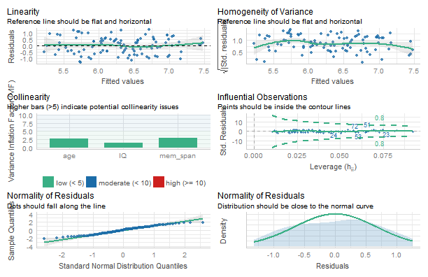<!-- --> --- # Normality of residuals ```r plot(check_normality(full_model)) ``` ``` ## OK: residuals appear as normally distributed (p = 0.060). ``` 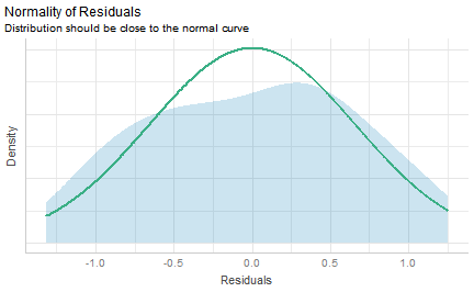<!-- --> --- # Normality of residuals ```r plot(check_normality(full_model), type = "qq") ``` ``` ## OK: residuals appear as normally distributed (p = 0.060). ``` <!-- --> --- # Checking for outliers ```r plot(check_outliers(full_model)) ``` <!-- --> --- # Heteroscedasticity ```r plot(check_heteroscedasticity(full_model)) ``` ``` ## OK: Error variance appears to be homoscedastic (p = 0.331). ``` <!-- --> --- # Multicollinearity A potential issue with multiple predictors is that they may be correlated with each other. Collinearity is a correlation between two predictors; multicollinearity is correlation between *two or more* predictors. Multicollinearity makes it harder to evaluate the individual contribution of a predictor to a model: it increases the estimated variability of correlated predictors. ```r cor(child_data[, c("IQ", "age", "mem_span")]) ``` ``` ## IQ age mem_span ## IQ 1.0000000 -0.1158099 0.3120912 ## age -0.1158099 1.0000000 0.7134009 ## mem_span 0.3120912 0.7134009 1.0000000 ``` --- # Multicollinearity .pull-left[ ```r plot(check_collinearity(full_model)) ``` [Graham, 2003. CONFRONTING MULTICOLLINEARITY IN ECOLOGICAL MULTIPLE REGRESSION](https://esajournals.onlinelibrary.wiley.com/doi/full/10.1890/02-3114) ] .pull-right[  ] --- # Reporting results ```r tab_model(full_model, show.std = TRUE) ``` <table style="border-collapse:collapse; border:none;"> <tr> <th style="border-top: double; text-align:center; font-style:normal; font-weight:bold; padding:0.2cm; text-align:left; "> </th> <th colspan="5" style="border-top: double; text-align:center; font-style:normal; font-weight:bold; padding:0.2cm; ">read_ab</th> </tr> <tr> <td style=" text-align:center; border-bottom:1px solid; font-style:italic; font-weight:normal; text-align:left; ">Predictors</td> <td style=" text-align:center; border-bottom:1px solid; font-style:italic; font-weight:normal; ">Estimates</td> <td style=" text-align:center; border-bottom:1px solid; font-style:italic; font-weight:normal; ">std. Beta</td> <td style=" text-align:center; border-bottom:1px solid; font-style:italic; font-weight:normal; ">CI</td> <td style=" text-align:center; border-bottom:1px solid; font-style:italic; font-weight:normal; ">standardized CI</td> <td style=" text-align:center; border-bottom:1px solid; font-style:italic; font-weight:normal; ">p</td> </tr> <tr> <td style=" padding:0.2cm; text-align:left; vertical-align:top; text-align:left; ">(Intercept)</td> <td style=" padding:0.2cm; text-align:left; vertical-align:top; text-align:center; ">2.96</td> <td style=" padding:0.2cm; text-align:left; vertical-align:top; text-align:center; ">-0.00</td> <td style=" padding:0.2cm; text-align:left; vertical-align:top; text-align:center; ">0.07 – 5.85</td> <td style=" padding:0.2cm; text-align:left; vertical-align:top; text-align:center; ">-0.15 – 0.15</td> <td style=" padding:0.2cm; text-align:left; vertical-align:top; text-align:center; "><strong>0.045</strong></td> </tr> <tr> <td style=" padding:0.2cm; text-align:left; vertical-align:top; text-align:left; ">mem span</td> <td style=" padding:0.2cm; text-align:left; vertical-align:top; text-align:center; ">0.64</td> <td style=" padding:0.2cm; text-align:left; vertical-align:top; text-align:center; ">0.29</td> <td style=" padding:0.2cm; text-align:left; vertical-align:top; text-align:center; ">0.06 – 1.23</td> <td style=" padding:0.2cm; text-align:left; vertical-align:top; text-align:center; ">0.03 – 0.56</td> <td style=" padding:0.2cm; text-align:left; vertical-align:top; text-align:center; "><strong>0.031</strong></td> </tr> <tr> <td style=" padding:0.2cm; text-align:left; vertical-align:top; text-align:left; ">age</td> <td style=" padding:0.2cm; text-align:left; vertical-align:top; text-align:center; ">0.31</td> <td style=" padding:0.2cm; text-align:left; vertical-align:top; text-align:center; ">0.40</td> <td style=" padding:0.2cm; text-align:left; vertical-align:top; text-align:center; ">0.11 – 0.50</td> <td style=" padding:0.2cm; text-align:left; vertical-align:top; text-align:center; ">0.15 – 0.66</td> <td style=" padding:0.2cm; text-align:left; vertical-align:top; text-align:center; "><strong>0.002</strong></td> </tr> <tr> <td style=" padding:0.2cm; text-align:left; vertical-align:top; text-align:left; ">IQ</td> <td style=" padding:0.2cm; text-align:left; vertical-align:top; text-align:center; ">-0.01</td> <td style=" padding:0.2cm; text-align:left; vertical-align:top; text-align:center; ">-0.07</td> <td style=" padding:0.2cm; text-align:left; vertical-align:top; text-align:center; ">-0.05 – 0.02</td> <td style=" padding:0.2cm; text-align:left; vertical-align:top; text-align:center; ">-0.26 – 0.12</td> <td style=" padding:0.2cm; text-align:left; vertical-align:top; text-align:center; ">0.477</td> </tr> <tr> <td style=" padding:0.2cm; text-align:left; vertical-align:top; text-align:left; padding-top:0.1cm; padding-bottom:0.1cm; border-top:1px solid;">Observations</td> <td style=" padding:0.2cm; text-align:left; vertical-align:top; padding-top:0.1cm; padding-bottom:0.1cm; text-align:left; border-top:1px solid;" colspan="5">100</td> </tr> <tr> <td style=" padding:0.2cm; text-align:left; vertical-align:top; text-align:left; padding-top:0.1cm; padding-bottom:0.1cm;">R<sup>2</sup> / R<sup>2</sup> adjusted</td> <td style=" padding:0.2cm; text-align:left; vertical-align:top; padding-top:0.1cm; padding-bottom:0.1cm; text-align:left;" colspan="5">0.419 / 0.401</td> </tr> </table> Tables can be particularly useful with multiple regression - especially with a lot of predictors. --- class: inverse, middle, center # Comparing multiple means with categorical predictors --- # Comparing the means of two groups Previously, we saw how to use `t.test()` to compare the means of two groups. ```r t.test(FoC ~ sex, data = crime, var.equal = TRUE) ``` ``` ## ## Two Sample t-test ## ## data: FoC by sex ## t = 4.7664, df = 299, p-value = 2.932e-06 ## alternative hypothesis: true difference in means between group female and group male is not equal to 0 ## 95 percent confidence interval: ## 0.3753039 0.9031487 ## sample estimates: ## mean in group female mean in group male ## 2.584681 1.945455 ``` --- # Comparing three or more means with ANOVA The `t.test()` can only handle two groups. When we have three or more groups, we need to use a One-Way Analysis of Variance (ANOVA). <!-- --> --- # How does ANOVA work? With a t-test, we typically ask the question "Is the difference between these two means significantly different from zero?" `$$\mu^1 \neq \mu^2$$` With an ANOVA, we ask the question "Are any of these means different from each other?" `$$\mu^1 \neq \mu^2 \neq \mu^3 ...$$` Another way to phrase this is "Do any of these means differ from the *grand* mean?" --- # The (grand) mean and the variance The *grand* mean is the mean across all conditions. ## A worked example .pull-left[ A researcher wants to examine the effect of noisy environments on test performance. She recruits 150 participants and splits them into three groups. One group performs the test without any environmental noise. A second group performs the test with fairly quiet noise. A third group performs the test with loud noise. The dependent variable is their score (out of 10) on the test. ] .pull-right[ ```r noise_test <- gather(tibble(none = rnorm(50, 8, 1), quiet = rnorm(50, 7, 1), loud = rnorm(50, 5, 1)), noise, test_score) %>% mutate(participant = 1:150) ``` ] --- # How the data is structured .pull-left[ ```r noise_test ``` ``` ## # A tibble: 150 x 3 ## noise test_score participant ## <chr> <dbl> <int> ## 1 none 6.97 1 ## 2 none 6.63 2 ## 3 none 8.10 3 ## 4 none 8.35 4 ## 5 none 7.14 5 ## 6 none 7.26 6 ## 7 none 8.34 7 ## 8 none 9.00 8 ## 9 none 6.33 9 ## 10 none 8.48 10 ## # ... with 140 more rows ``` ] .pull-right[ One column per variable! One column - *noise* - is the categorical predictor variable that tells which group each participant was in. One column - *test_score* - is the dependent variable. The final column - participant - is a (unique - each participant always has the same identifier) participant identifier. ] --- # The mean as a model (again) We went through this in detail last time, but here's how it applies here. The simplest model of this data is to use the grand mean across all conditions. .pull-left[ <!-- --> ] .pull-right[ The grand mean test score is 6.54, shown by the black line. The total variability in our data is the sum of the squared differences from the grand mean - the Total Sum of Squares, `\(SS_t\)`. ] --- # The group means as a model The model we're interested in is the means as a function of group. .pull-left[ <!-- --> ] .pull-right[ Our Model Sum of Squares - `\(SS_m\)` - is the sum of the squared differences of each group's mean from the *grand mean*. The group means are shown here using coloured lines. The final quantity, the Residual Sum of Squares - `\(SS_r\)` is the sum of the squared differences of each individual observation from the mean of the group to which it belongs. ] --- # Degrees of freedom .large[ We now have measures of the total amount of variability explained by the data, the total amount explained by our model, and the amount left over by our model. However, these numbers are biased because different amounts of values went into their calculation - 3 were used to calculate the `\(SS_m\)`, while many more were used to calculate `\(SS_t\)` and `\(SS_r\)`. We correct these using the *degrees of freedom*. Specifically, we need to correct `\(SS_r\)` and `\(SS_m\)` with the residual degrees of freedom - `\(df_r\)` and the model degrees of freedom - `\(df_m\)`. ] --- # Degrees of freedom .large[ The model degrees of freedom is simply the number of groups - 1; where *k* = number of groups: `$$df_m = k - 1$$` The residual degrees of freedom is the sum of all the degrees of freedom for each group. `$$df_r = \sum{df_{group^k}}$$` ] --- # Mean squared error and the F-ratio Finally, we divide our sums of squares - `\(SS_m\)` and `\(SS_r\)` by `\(df_m\)` and `\(df_r\)` respectively, giving us the mean squared error of the model - `\(MS_m\)` - and mean squared error of the residuals - `\(MS_r\)`. `$$MS_m = \frac{SS_m}{df_m}$$` `$$MS_r = \frac{SS_r}{df_r}$$` The ratio of these two quantities is the *F-ratio*. `$$F = \frac{MS_m}{MS_r}$$` In English, the F-ratio is the ratio of the variability explained by the model to variability unexplained by the model. So, higher is better. --- class: inverse, center, middle # How to run a one-way between subjects ANOVA --- # How to run ANOVA with the *afex* package Although the standard R function for ANOVA, `aov()`, works, it can be fiddly to use. The `afex` package provides several easier methods for running ANOVA. We'll use the `aov_ez()` function. ```r noise_aov <- aov_ez(dv = "test_score", between = "noise", id = "participant", data = noise_test) ``` ``` ## Converting to factor: noise ``` ``` ## Contrasts set to contr.sum for the following variables: noise ``` --- # Checking the results ```r noise_aov ``` ``` ## Anova Table (Type 3 tests) ## ## Response: test_score ## Effect df MSE F ges p.value *## 1 noise 2, 147 1.09 115.39 *** .611 <.001 ## --- ## Signif. codes: 0 '***' 0.001 '**' 0.01 '*' 0.05 '+' 0.1 ' ' 1 ``` There's a highly significant effect of the factor *noise*. But ANOVA only tells us that there is a difference; not what the difference is! --- # Follow-up contrasts We can use the `emmeans` package to get more information about our results. First, let's run the `emmeans()` function to get the means for each condition. ```r means_noise <- emmeans(noise_aov, ~noise) means_noise ``` ``` ## noise emmean SE df lower.CL upper.CL ## loud 4.80 0.147 147 4.51 5.09 ## none 7.90 0.147 147 7.61 8.19 ## quiet 6.92 0.147 147 6.63 7.22 ## ## Confidence level used: 0.95 ``` It looks like performance was best is when there was no noise, with the worst performance when there was loud noise. --- # Follow-up contrasts After calculating the means, we can then compare all of the means to each other using the `pairs()` function. ```r pairs(means_noise) ``` ``` ## contrast estimate SE df t.ratio p.value ## loud - none -3.097 0.209 147 -14.853 <.0001 ## loud - quiet -2.124 0.209 147 -10.188 <.0001 ## none - quiet 0.973 0.209 147 4.665 <.0001 ## ## P value adjustment: tukey method for comparing a family of 3 estimates ``` Note that this corrects the p-values for multiple comparisons. There are three possible comparisons, each with a significance threshold of p = .05; the more possible comparisons, the more you have to correct for false positives. --- # Visualizing the results As ever, it's best to support your inferences with visualizations. `afex_plot()` from the `afex` package can automatically create plots from the fitted ANOVA. ```r afex_plot(noise_aov, x = "noise") + theme_classic() ``` <!-- --> --- # Assumptions of ANOVA Just like the t-test and our linear regressions, normality of the model residuals is assumed. We can check that with the `check_normality()` function from the `performance` package. ```r library(performance) plot(check_normality(noise_aov)) ``` ``` ## OK: residuals appear as normally distributed (p = 0.605). ``` <!-- --> --- # Assumptions of ANOVA **Homogeneity of variance is also assumed**. This can be explicitly tested using the `check_homogeneity()` function from the `performance` package. ```r plot(check_homogeneity(noise_aov)) ``` ``` ## OK: There is not clear evidence for different variances across groups (Levene's Test, p = 0.649). ``` <!-- --> --- # Assumptions of (between-subjects) ANOVA Each observation should be independent - i.e. there should be no repeated measures. Each participant is in one group and one group only, and contributes one data point to that group. --- # Next week Repeated-measures ANOVA. Factorial and mixed ANOVA. These are covered in chapters 12-14 of Discovering Statistics Using R.