Linear Modelling
Matt Craddock
2024-08-15
Source:vignettes/linear_modelling/linear_modelling.Rmd
linear_modelling.Rmd
library(eegUtils)
#>
#> Attaching package: 'eegUtils'
#> The following object is masked from 'package:stats':
#>
#>     filter
library(R.matlab)
#> R.matlab v3.7.0 (2022-08-25 21:52:34 UTC) successfully loaded. See ?R.matlab for help.
#>
#> Attaching package: 'R.matlab'
#> The following objects are masked from 'package:base':
#>
#>     getOption, isOpen
library(ggplot2)
library(tidyr)
Here we show how to fit a linear model to a single subject’s data. We’ll use the data from the LIMO EEG datase [^1] - S1
This data is from a two-alternative forced choice experiment in which participants had to discriminate between two different faces. Across the course of the experiment, the faces were also varied in their phase coherence from 0% to 85%. The more phase coherent the face images, the easier they were to discriminate from each other.
limo_test <- import_set("limo_dataset_S1.set")
#> Importing from EEGLAB .set file.
#> Importing data from .fdt file.
#> Rounding non-integer event sample latencies...
limo_cont <- R.matlab::readMat("continuous_variable.mat")
limo_cat <- readr::read_csv("categorical_variable.txt",
                            col_names = c("cond_lab"))
#> Rows: 1055 Columns: 1
#> ── Column specification ────────────────────────────────────────────────────────
#> Delimiter: ","
#> dbl (1): cond_lab
#>
#> ℹ Use `spec()` to retrieve the full column specification for this data.
#> ℹ Specify the column types or set `show_col_types = FALSE` to quiet this message.
The fit_glm() linear model fitting function in
eegUtils looks in the epochs field of the data
structures as predictors. To use these for linear modelling here, we’ll
add the categorical and continuous predictors to the epochs
structure.
epochs(limo_test) <- dplyr::mutate(epochs(limo_test),
                            phase_coherence = unlist(limo_cont),
                            face = factor(limo_cat$cond_lab,
                                          levels = c(1, 2),
                                          labels = c("Face_A",
                                                     "Face_B")))
epochs(limo_test)
#> # A tibble: 1,055 × 5
#>    epoch participant_id  recording       phase_coherence face
#>    <int> <chr>           <chr>                     <dbl> <fct>
#>  1     1 limo_dataset_S1 limo_dataset_S1            0.6  Face_B
#>  2     2 limo_dataset_S1 limo_dataset_S1            0.55 Face_A
#>  3     3 limo_dataset_S1 limo_dataset_S1            0.3  Face_B
#>  4     4 limo_dataset_S1 limo_dataset_S1            0.1  Face_A
#>  5     5 limo_dataset_S1 limo_dataset_S1            0.15 Face_A
#>  6     6 limo_dataset_S1 limo_dataset_S1            0.1  Face_B
#>  7     7 limo_dataset_S1 limo_dataset_S1            0.85 Face_A
#>  8     8 limo_dataset_S1 limo_dataset_S1            0.8  Face_B
#>  9     9 limo_dataset_S1 limo_dataset_S1            0.25 Face_A
#> 10    10 limo_dataset_S1 limo_dataset_S1            0.65 Face_B
#> # ℹ 1,045 more rows
The first argument to fit_glm() is a standard R formula,
using Wilkinson notation. Unusually, the left hand side of the
~ is omitted, since we’ll be fitting the model to every
electrode at every timepoint. On the right hand side, we put our
predictors. In this case, we have two: face, a categorical
predictor; and phase_coherence, a continuous predictor. The
appropriate formula is thus ~face + phase_coherence.
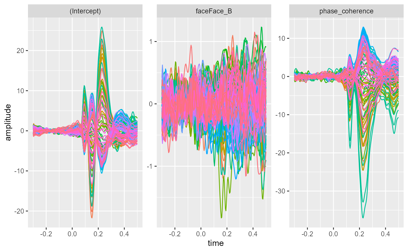
R’s default contrasts are treatment or dummy
contrasts, so we expect the model to return three coefficients: an
intercept, which will be the amplitude when the categorical
predictor is at its first level (i.e. Face A) and when phase coherence
is 0; a face term, which will be the difference in
amplitude from the intercept when the level of Face is
Face B; and a phase_coherence term, which will be
the increase in amplitude when image phase coherence increases from 0 to
1.
We can convert the fitted model into a standard data.frame using the
as.data.frame function. By default, this returns the
coefficients for each time point for each electrode. The
values argument can be used to request other statistics by
passing “coefficients”, “std_err”, “t_stats”, or “r_sq”.
fitted_model <- fit_glm(~ face + phase_coherence,
                        data = limo_test)
as.data.frame(fitted_model,
              long = TRUE) %>%
  ggplot(aes(x = time,
             y = amplitude,
             colour = electrode)) +
  geom_line() +
  facet_wrap(~coefficient,
             scales = "free") +
  theme(legend.position = "none")
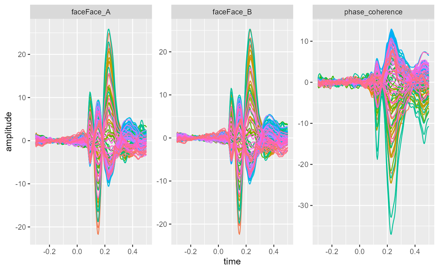
An alternative paramterization would be to remove the intercept term.
The function would then return separate coefficients representing
Face A and Face B. This would be particularly
helpful if you are planning to take these coefficients forwards to a
second-level analysis.
fitted_model_no_int <- fit_glm(~0 + face + phase_coherence,
                        data = limo_test)
as.data.frame(fitted_model_no_int,
              long = TRUE) %>%
  ggplot(aes(x = time,
             y = amplitude,
             colour = electrode)) +
  geom_line() +
  facet_wrap(~coefficient,
             scales = "free") +
  theme(legend.position = "none")
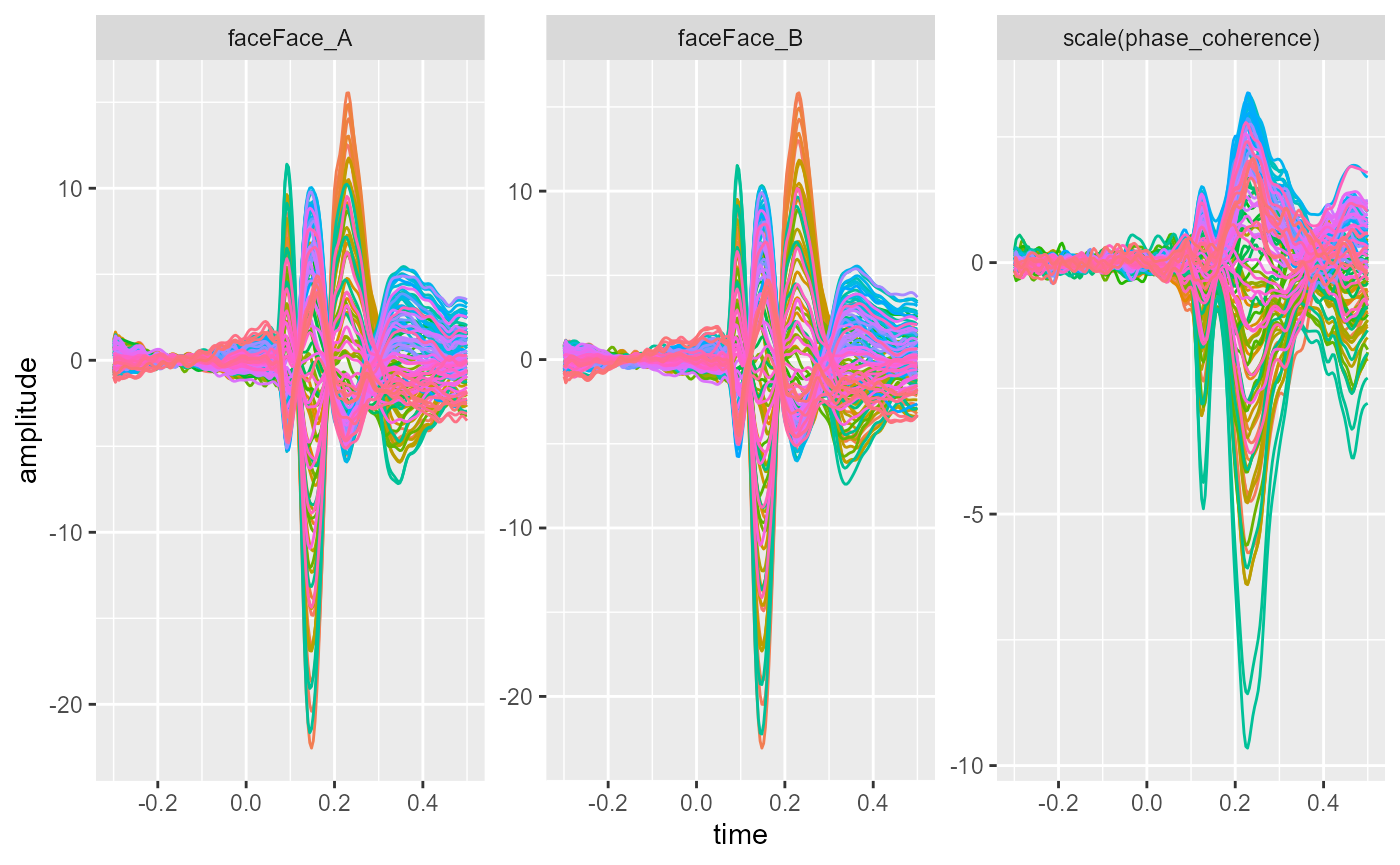
Continuous predictors can be rescaled using the scale()
function, which converts them to z-scores (i.e. standard deviation
units).
fitted_model_zscore <- fit_glm(~0 + face + scale(phase_coherence),
                        data = limo_test)
as.data.frame(fitted_model_zscore,
              long = TRUE) %>%
  ggplot(aes(x = time,
             y = amplitude,
             colour = electrode)) +
  geom_line() +
  facet_wrap(~coefficient,
             scales = "free") +
  theme(legend.position = "none")
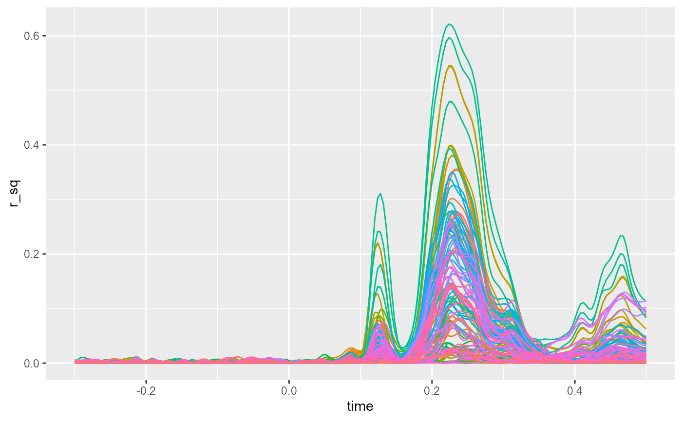
The function also provide additional information. For example, we can get the value representing model fit:
fitted_model$r_sq %>%
  pivot_longer(cols = channel_names(limo_test),
               names_to = "electrode",
               values_to = "r_sq") %>%
  ggplot(aes(x = time,
             y = r_sq,
             colour = electrode)) +
  geom_line() +
  theme(legend.position = "none")
References
[^1] Guillaume, Rousselet. (2016). LIMO EEG Dataset, [dataset]. University of Edinburgh, Centre for Clinical Brain Sciences. https://doi.org/10.7488/ds/1556.